Previous article: Estimation Crash Course I: Statistics and Estimators
Next article: Estimation Crash Course III: The Cramér-Rao bound
Fisher Information for one-parameter models
We shall introduce the concept of the Fisher information via an example. Let $X\sim\mathcal{N}(\mu, \sigma^2)$ where $\sigma^2$ is known and $\mu$ is unknown. Let us consider two cases:
- Case I: $X\sim\mathcal{N}(\mu, 20)$ (large variance),
- Case II: $X\sim\mathcal{N}(\mu, 0.1)$ (small variance),
where the value of $\mu$ is the same in both cases. Suppose we obtain one measurement, $X=x$, so the log-likelihood of $\mu$ is
$$\ell(\mu; x) = \log p_X(x; \mu) = -\log(\sqrt{2\pi} \sigma) -\frac{(x-\mu)^2}{2\sigma^2}.\tag{1}$$
Figure 1 shows the log-likelihood functions, $\ell(\mu; x)$, for a few samples $X\sim\mathcal{N}(\mu, 0.1)$ (Case I). We can say that each observation is quite informative about the parameter $\mu$.
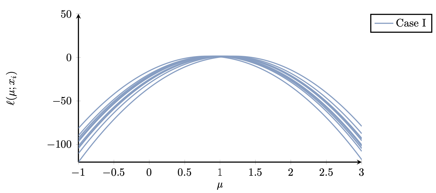
Figure 1. (Case I) Plot of $\ell(\mu; x_i)$ for $N=20$ measurements. The likelihood function has, on average, a healthy curvature (it is not too flat).
It is not difficult to guess the true value of $\mu$ from the above plot (in fact it is $\mu=1$). On the other hand, in Case II we have the following plot (Figure 2) of the log-likelihood function for each observation
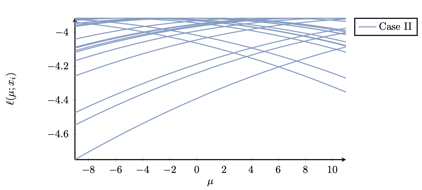
Figure 2. (Case II) Plot of $\ell(\mu; x_i)$ for $N=20$ measurements. The likelihood function is, on average, quite flat.
Here it is more difficult to guess what the true value of $\mu$ is, or, to put it differently, the data are less informative about $\mu$, the main reason being that
Fisher proposed the following quantity to quantify the information that an observation $X$ (or several observations, $X_1,\ldots, X_N$) offers about the parameter $\theta$:
$$I(\theta) {}={} -{\rm I\!E}\left[ \left. \frac{\partial^2}{\partial \theta^2}\ell(\theta; X) \right| {}\theta \right],\tag{2}$$
where the expectation is taken with respect to $X$ and $\ell$ denotes the log-likelihood. In other words, using the pdf of $X$,
$$ I(\theta) {}={} \int_E \frac{\partial^2}{\partial \theta^2}\ell(\theta; x)p_X(x; \theta){\rm d} x.\tag{3}$$
This quantity is known as the Fisher information of the statistical model. The Fisher information quantifies how much information the data gives us for the unknown parameter.
There is an alternative expression for the determination of $I(\theta)$ --- we will prove it in a moment --- which uses the first derivative of $\ell$:
$$I(\theta) {}={} {\rm I\!E}\left[ \left. \left(\frac{\partial \ell(\theta; X)}{\partial \theta}\right)^2 \right| {}\theta \right].\tag{4}$$
Again, as we did in Equation (3), we can use the pdf of $X$ to compute $I(\theta)$, that is,
$$I(\theta) {}={} \int_E \left(\frac{\partial \ell(\theta; x)}{\partial \theta}\right)^2 p_X(x; \theta){\rm d} x.\tag{5}$$
The Fisher information is defined if the following basic regularity conditions are satisfied: (i) $p_X(x; \theta)$ is differentiable wrt $\theta$ almost everywhere, (ii) the support of $p_X(x; \theta)$ does not depend on $\theta$. In other words, the set $\{x{}:{} p_X(x;\theta)>0\}$ does not depend on $\theta$, and (iii) it holds that $\frac{\partial}{\partial \theta}\int p_X(x;\theta){\rm d} x = \int \frac{\partial}{\partial \theta} p_X(x;\theta){\rm d} x$.
Note that the first assumption is not satisfied for the uniform distribution, $U(0, \theta)$, and the Fisher information is not defined for $U(0, \theta)$.
Theorem 1 (Fisher Information Equivalent Formulas). Suppose $\ell(\theta; X)$ is the likelihood of a parameter $\theta$ given some observation(s) $X$ and the above regularity assumptions are satisfied. Then,
$${\rm I\!E}\left[ \left. \frac{\partial \ell(\theta; X)}{\partial \theta} \right| {}\theta \right] = 0.\tag{6}$$
Additionally, assume that it is twice differentiable and (iv) assumption (iii) holds for the second order derivative wrt $\theta$. Then, the Fisher information is given by
$$\begin{aligned}I(\theta) {}={}& -{\rm I\!E}\left[ \left. \frac{\partial^2}{\partial \theta^2}\ell(\theta; X) \right| {}\theta \right]\\ {}={}& {\rm I\!E}\left[ \left. \left(\frac{\partial \ell(\theta; X)}{\partial \theta}\right)^2 \right| {}\theta \right] {}={} {\rm Var}\left[ \left. \frac{\partial \ell(\theta; X)}{\partial \theta} \right| {}\theta \right] \tag{7}.\end{aligned}$$
Note. The quantity $\frac{\partial \ell(\theta; X)}{\partial \theta}$ is called the score function. The mean score is zero, while the variance of the score is the Fisher information.
Proof. We have
$$\begin{aligned} {\rm I\!E}\left[ \left. \frac{\partial \ell(\theta; X)}{\partial \theta} \right| {}\theta \right] {}={} & {\rm I\!E}\left[ \left. \frac{\partial \log p(X; \theta)}{\partial \theta} \right| {}\theta \right] {}={} \int_E \frac{\frac{\partial p_X(x; \theta)}{\partial \theta}}{\cancel{p_X(x; \theta)}}\cancel{p_X(x; \theta)}{\rm d} x \\ {}={} & \int_E \frac{\partial p_X(x; \theta)}{\partial \theta}{\rm d} x {}\overset{\text{Ass.~(iii)}}{=}{} \frac{\partial}{\partial \theta} \underbrace{\int_E p_X(x; \theta) {\rm d} x}_{=1} = 0,\tag{8} \end{aligned}$$
so the last equality in Equation (7) follows.
To prove that the two expectations are equal we use the fact that
$$\begin{aligned} \frac{\partial^2}{\partial \theta^2}\log p_X(X; \theta) {}={}& \frac{\frac{\partial^2 p_X(X; \theta)}{\partial \theta^2}}{p_X(X; \theta)} {}-{} \left(\frac{\frac{\partial^2 p_X(X; \theta)}{\partial \theta^2}}{p_X(X; \theta)}\right)^2 \\ {}={}& \frac{\frac{\partial^2 p_X(X; \theta)}{\partial \theta^2}}{p_X(X; \theta)} {}-{} \left( \frac{\partial}{\partial \theta}\log p_X(X; \theta) \right)^2.\tag{9}\end{aligned}$$
Note that
$$\begin{aligned}{\rm I\!E}\left[\frac{\frac{\partial^2 p_X(X; \theta)}{\partial \theta^2}}{p_X(X; \theta)}\right] {}={}& \int_E \frac{\frac{\partial^2 p_X(x; \theta)}{\partial \theta^2}}{\cancel{p_X(x; \theta)}} \cancel{p_X(x; \theta)} {\rm d} x \\ {}\overset{\text{(iv)}}{=}{}& \frac{\partial^2 p_X(x; \theta)}{\partial \theta^2} \underbrace{\int_E p_X(x;\theta){\rm d} x}_{=1}=0.\tag{10}\end{aligned}$$
Now taking the expectation on Equation (9) and using Equation (10), Equation (7) follows. $\Box$
Example 1 (Fisher information of Exponential). Suppose $X{}\overset{\text{iid}}{=} {} {\rm Exp}(\lambda)$ where $\lambda>0$ is an unknown value. We want to quantify how informative a measurement of $X$. The likelihood function is $L(\lambda, x) = \lambda e^{-\lambda x}$, where $x\geq 0$, so the log-likelihood is $\ell(\lambda, x) = \log \lambda - x\lambda$. Suppose that the true value of $\lambda$ is $3$. Let us samples some values $x_1,\ldots, x_10$ using Python (numpy.random.Generator.exponential) and plot $\ell(\lambda, x_i)$ which is shown in Figure 3.
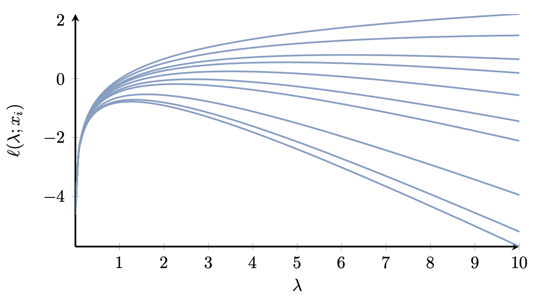
Figure 3. Log-likelihood, $\ell(\lambda; x_i)$, for different values sampled from ${\rm Exp}(3)$.
In this example we see that the log-likelihood is not quadratic in $\lambda$, so its curvature depends on $\lambda$. In particular, the curvature is
$$\frac{\partial^2 }{\partial \lambda^2}\ell(\lambda; X) = -\frac{1}{\lambda^2},\tag{11}$$
therefore, the Fisher information is $I(\lambda) = -\frac{1}{\lambda^2}$. $\heartsuit$
Example 2 (Fisher information of Bernoulli). The likelihood function of a Bernoulli trial is $L(p; X) = p^X (1-p)^{1-X}$, so the log-likelihood is
$$\ell(p; X) = X\log p + (1-X)\log(1-p)\tag{12}$$
The second derivative of $\ell$ with respect to $p$ is
$$\frac{\partial^2 \ell(p; X)}{\partial p^2} {}={} \frac{X}{p^2} + \frac{1-X}{(1-p)^2}.\tag{13}$$
The Fisher information is
$$I(p) {}={} {\rm I\!E}\left[\left.\frac{\partial^2 \ell(p; X)}{\partial p^2}\right| p \right] {}={} {\rm I\!E}\left[\left.\frac{X}{p^2} + \frac{1-X}{(1-p)^2}\right| p \right] = \ldots = \frac{1}{p(1-p)}.\tag{14}$$
The plot of the Fisher information, $I(p)$, is shown in Figure 4.
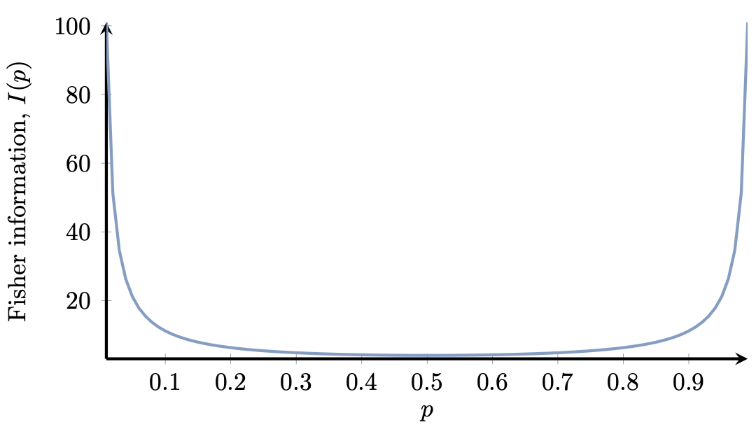
Figure 4. Fisher information for ${\rm Ber}(p)$ as a function of $p$. The outcomes of blatantly unfair coins are more informative about the parameter $p$.
We see that the Fisher information increases for values of $p$ close to $0$ or $1$ (for blatantly unfair coins). $\heartsuit$
Example 3 (Normal with known variance). Consider the random variable $X\sim\mathcal{N}(\mu, \sigma^2)$, with known variance and unknown mean. It is not difficult to see that
$$I(\mu) = \frac{1}{\sigma^2}.$$
As one would expect, the higher the variance, the lower the Fisher information (the less informative each observation is about the mean). Note, that the Fisher information in this case does not depend on the parameter.
Exercises
Exercise 1. Determine the Fisher information in each of the following cases:
- ${\rm Poisson}(\lambda)$
- ${\rm Exp}(\lambda)$
- $\mathcal{N}(\mu, \sigma^2)$ with known $\sigma^2$
- $\mathcal{N}(0, \sigma^2)$ with unknown $\sigma^2$
For each of the above distributions, plot $I(\theta)$ and produce figures akin to Figure 1 or Figure 3 for different values of $\theta$.
Exercise 2 Suppose that the Fisher information associated with a likelihood function $\ell(\theta; X)$ is $I(\theta)$. Suppose we have a sample of $N$ observations, $X_1,\ldots, X_N$. Show that the Fisher information for $\ell(\theta;X_1,\ldots, X_N)$ is $NI(\theta)$.
Exercise 3 (Fisher information of transformation). Suppose the log-likelihood function, $\ell(\theta; X)$, has Fisher information $I(\theta)$. Now suppose that the statistical model is parametrised with a parameter $\lambda$ such that $\theta = g(\lambda)$, for some continuously differentiable function $g$. Let $I_1(\lambda)$ be the Fisher information of the new model. Show that
$$I_1(\lambda) = g'(\lambda)^2 I(g(\lambda)).$$
Exercise 4 (Application of Exercise 3). Suppose $X\sim{\rm Exp}(\lambda)$. We know that the Fisher information is $I(\lambda)=1/\lambda^2$. We reparametrise this model using $\lambda = \xi^2$, that is $X\sim{\rm Exp}(\xi^2)$. What is the Fisher information of the parameter $\xi$ for the new model?
Reparametrisation and Fisher information
The Fisher information depends on the parametrisation of the model. For instance, let us go back to Example 3, but now let us assume that $\mu = 1/\tau$, where $\tau\neq 0$ is a new parameter. The reader can verify that the Fisher information of $\tau$ is
$$I(\tau) = \frac{1}{\sigma^2 \tau^4}.$$
To avoid confusion, from now on let us denote the Fisher information with respect to a parameter $\theta$, by $I_{\theta}$.
Theorem 2 (Reparametrisation of Fisher information). Consider a statistical model involving a parameter $\theta\in\Theta \subseteq {\rm I\!R}$ and a sample $X$ with pdf $p(x; \theta)$. Let $I_\theta(\theta)$ be the Fisher information of $\theta$. The Fisher information of the parametrisation $\theta = \phi(u)$, where $\phi$ is a differentiable function, is given by
$$I_u(u) = \phi'(u)^2 I_\theta(\phi(u)).$$
Proof. The log-likelihood with respect to $u$ is $\ell(\phi(u); X)$ and its derivative with respect to $u$ is
$$\frac{{\rm d}}{{\rm d}u}\ell(\phi(u); X) = \phi'(u) \ell'(\phi(u), X).$$
By employing Theorem 1 the proof is complete. $\Box$
Multivariate models
Where $\theta \in {\rm I\!R}^n$ is a vector, the Fisher information is defined to be an $n\times n$ matrix given by
$$[I(\theta)]_{i,j} = -{\rm I\!E}\left[\frac{\partial^2}{\partial \theta_i \partial \theta_j}\ell(X; \theta)\right],$$
for $i,j=1,\ldots, n$, or, what is the same,
$$I(\theta) = -{\rm I\!E}\left[\nabla_\theta^2 \ell(X; \theta)\right].$$
In the multivariate case, the score function is defined as
$$s(\theta)_i = \frac{\partial}{\partial \theta_i}\ell(X; \theta),$$
for $i=1,\ldots, n$, or, what is the same
$$s(\theta) = \nabla_\theta \ell(X; \theta).$$
Similar to what we showed in Theorem 1, we can show that
$$I(\theta) = {\rm Var}[s(\theta)] = {\rm I\!E}[s(\theta)s(\theta)^\intercal].$$
Example 4 (Normal distribution). Consider the case where $X$ follows the normal distribution, $X\sim\mathcal{N}(\mu, \sigma^2)$, and both $\mu$ and $\sigma^2$ are unknown. Let us choose the parameter vector $\theta=(\mu, \sigma^2)$. Then, the log-likelihood function is
$$\ell(\theta; x) = -\frac{1}{2}\log(2\pi\sigma^2) - \frac{1}{2\sigma^2}(x-\mu)^2.$$
The score function is
$$s(\theta; X) = \nabla_\theta \ell(\theta; X) = \begin{bmatrix} \frac{X-\mu}{\sigma^2} \\[1em] \frac{(X-\mu)^2}{2\sigma^4} - \frac{1}{2\sigma^2} \end{bmatrix}$$
We can then determine the Fisher information matrix
$$I(\mu, \sigma^2) = \begin{bmatrix} \frac{1}{\sigma^2} \\ & \frac{1}{2\sigma^4}\end{bmatrix}.$$
Read next: Estimation Crash Course III: The Cramér-Rao bound