This is the first post of a series on the Kalman filter. We will start simply by stating a linear dynamical system, without an input, which is subject to Gaussian process noise, and we will study its properties.
Read next: Kalman Filter II: Conditioning
The Gauss-Markov Model
Consider the linear dynamical system (without an input)
$$\begin{aligned}x_{t+1} {}={} & A_t x_t + G_t w_t,\\y_t {}={} & C_t x_t + v_t,\end{aligned}$$
where $x_t\in{\rm I\!R}^{n_x}$ is the system state, $y_t\in{\rm I\!R}^{n_y}$ is the output, $w_t\in{\rm I\!R}^{n_w}$ is a noise term acting on the system dynamics known as process noise, and $v_t\in{\rm I\!R}^{n_v}$ is a measurement noise term.
Assumptions
We assume that
- ${\rm I\!E}[w_t]=0$ and ${\rm I\!E}[v_t]=0$ for all $t\in{\rm I\!N}$,
- $x_0$, $(w_t)_t$ and $(v_t)_t$ are mutually independent random variables (therefore, ${\rm I\!E}[w_tw_l^\intercal]=0$ for $t{}\neq{}l$, and ${\rm I\!E}[v_tv_l^\intercal]=0$ for $t{}\neq{}l$),
- $w_t$ and $v_t$ are normally distributed and ${\rm I\!E}[w_tw_t^\intercal]=Q_t$, ${\rm I\!E}[v_tv_t^\intercal]=R_t$.
- $x_0$ is a random variable and $x_0 \sim \mathcal{N}(\tilde{x}_0, P_0)$
Example
As an example, consider the system
$$x_{t+1} = \begin{bmatrix}\phantom{-}0.5& 0.3\\ -0.2& 0.5\end{bmatrix}x_t + w_t,$$
where
$$w_t \sim \mathcal{N}\left(\begin{bmatrix}0\\0\end{bmatrix}, \begin{bmatrix}0.10& 0.05\\ 0.05& 0.15\end{bmatrix}\right),$$
and the initial condition:
$$x_0\sim\mathcal{N}\left(\begin{bmatrix}\phantom{-}5\\ -1\end{bmatrix}, \begin{bmatrix}0.9 & 0.4\\0.4& 0.3\end{bmatrix}\right).$$
The evolution of the system states - which are random variables - starting from the above initial condition is illustrated below.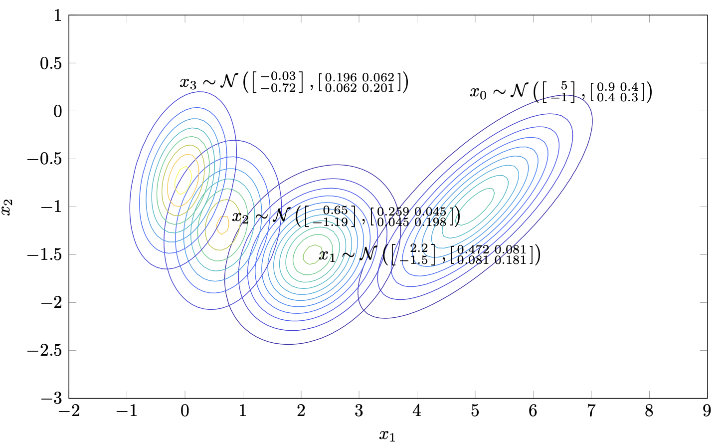
Figure I.1. Evolution of states of the Gauss-Markov model.
Evolution of expectation and variance
For the system in Figure I.1, define $\tilde{x}_t = {\rm I\!E}[x_t]$. Then,
$$\begin{aligned}\tilde{x}_{t+1} {}={} & {\rm I\!E}[x_{t+1}] = {\rm I\!E}[A_tx_{t} + G_tw_t] {}={} A_t {\rm I\!E}[x_t] {}={} A_t \tilde{x}_t.\end{aligned}$$
Define $P_{t} = \mathrm{Var}[x_t]$. Then,
$$\begin{aligned} P_{t+1} {}={} & {\rm I\!E}\Big[(x_{t+1} - \tilde{x}_{t+1})(x_{t+1} - \tilde{x}_{t+1})^\intercal\Big] \\ {}={} & {\rm I\!E}\Big[(A_tx_t + G_tw_t - A_t\tilde{x}_t)(A_tx_t + G_tw_t - A_t\tilde{x}_t)^\intercal\Big] \\ {}={} & {\rm I\!E}\Big[(A_t(x_t-\tilde{x}_t) + G_tw_t)(A_t(x_t-\tilde{x}_t) + G_tw_t)^\intercal\Big] \\ {}={} & {\rm I\!E}\Big[ A_t(x_t-\tilde{x}_t)(x_t-\tilde{x}_t)^\intercal{}A_t^\intercal {}+{} 2A_t(x_t-\tilde{x}_t)w_t^\intercal G_t^\intercal {}+{} G_tw_tw_t^\intercal{}G_t^\intercal \Big] \\ {}={} & A_t P_t A_t^\intercal + G_t{}Q_t{}G_t^\intercal, \end{aligned}$$
So the variance-covariance matrix of the state evolves according to
$$ P_{t+1} = A_t P_t A_t^\intercal + G_t{}Q_t{}G_t^\intercal. $$
It is reasonable to ask what happens as $t\to\infty$. For simplicity assume that $A_t = A$, $Q_t = Q$ and $G_t = G$ for all $t$. Then we have the update equation $P_{t+1} = AP_t A^{\intercal} + GQG^\intercal$. We know that if $A$ is a stable matrix (i.e., has a spectral radius less than $1$), then for every symmetric positive semidefinite $P_0$, the sequence $(P_t)_t$ converges to a matrix $P$ that satisfies the Lyapunov equation $P = A^\intercal P A + GQG^\intercal$. This matrix in the above example can be computed using MATLAB's dlyap to get
$$P = \begin{bmatrix}0.1858 & 0.0740 \\ 0.0740 & 0.1902\end{bmatrix}.$$
Markovianity of the state sequence
The sequence of states is Markovian, that is,
$$p_{x_{t+1}{}\mid{} x_0, x_1, \ldots, x_{t}}(x_{t+1} {}\mid{} x_0, x_1, \ldots, x_{t}) {}={} p_{x_{t+1}{}\mid{} x_{t}}(x_{t+1} {}\mid{} x_{t}).$$
This property suggests that the next state, $x_{t+1}$, can be estimated equally well if we know just $x_t$ as compared to knowing all the states $x_0, \ldots, x_t$. In other words, we do not need to condition by the whole history of states.
Proof. To prove this equality of probability density functions (pdfs) we will try to show that the corresponding cumulative distribution functions (cdfs) are equal. We have
$$\begin{aligned} F_{x_{t+1}{}\mid{} x_0, x_1, \ldots, x_{t}}(x^+ {}\mid{} x_0, x_1, \ldots, x_{t}) {}={}& {\sf P}[x_{t+1} \leq x^+ {}\mid{} x_0, x_1, \ldots, x_{t}] \\ {}={}& {\sf P}[Ax_{t} + w_t \leq x^+ {}\mid{} x_0, x_1, \ldots, x_{t}] \\ {}={}& {\sf P}[Ax_{t} + w_t \leq x^+ {}\mid{} x_{t}], \end{aligned}$$
where the last equality is because of the independence assumptions we stated earlier. $\Box$
Note that the sequence of output is not Markovian.
A key property towards the Kalman filter
A property that plays a key role in the development of the Kalman filter is
Proposition I.1 (Key result). It is $$p_{x_{t+1}\mid x_t}(x_{t+1}\mid x_t) {}={} p_{w_t}(x_{t+1} - Ax_t).$$
This can be easily generalised when the system is nonlinear, but let us prove this first.
Proof. It suffices to prove that the corresponding cumulative distribution functions are equal. We have
$$\begin{aligned}F_{x_{t+1}{}\mid x_t}(x^+) = {\sf P}[x_{t+1} \leq x^+ {}\mid{} x_t] =& {\sf P}[Ax_{t} + w_t \leq x^+ {}\mid{} x_t] \\ =& {\sf P}[ w_t \leq x^+ - Ax_{t} {}\mid{} x_t] \\ =& F_{w_t}(x^+ - Ax_{t}).\end{aligned}$$
Differentiating with respect to $x^+$ completes the proof. $\Box$
Covariances
We will determine ${\rm Cov}(x_t, x_{t+l}) = {\rm I\!E}[(x_t - \tilde{x}_t)(x_{t+l} - \tilde{x}_{t+1})^{\intercal}]$. The covariance has the following properties: for two random variables $X$, $Z$, $S$ and matrix $A$,
- ${\rm Cov}(X,X) = {\rm Var}(X)$
- ${\rm Cov}(X, Y) = {\rm Cov}(Y, X)^\intercal$
- ${\rm Cov}(AX, Z) = A{\rm Cov}(X, Z)$
- ${\rm Cov}(X, AZ) = {\rm Cov}(X, Z)A^\intercal$
- If $X$ and $Z$ are independent, ${\rm Cov}(X, Z) = 0$
- ${\rm Cov}(X, Z + S) = {\rm Cov}(X, Z) + {\rm Cov}(X, S)$
provided all covariances exist and are finite.
Let us assume for simplicity that $A_t = A$, $t\in{\rm I\!N}$. Then, for $l=1$ we have
$$\begin{aligned} {\rm Cov}(x_t, x_{t+1}) =& {\rm Cov}(x_t, Ax_t + w_t) \\ =& {\rm Cov}(x_t, Ax_t) + {\rm Cov}(x_t, w_t) \\ =& {\rm Cov}(x_t, x_t) A^\intercal \\ =& P_t A^\intercal, \end{aligned}$$
where we used the assumption that $w_t$ is independent of $x_t$. It is not difficult to apply the same procedure recursively to see that for all $t,l\in{\rm I\!N}$$$ {\rm Cov}(x_t, x_{t+l}) = P_t (A^{\intercal})^l.$$
Read next: Kalman Filter II: Conditioning