Read first: Kalman Filter V: It’s BLUE!
Read next: Kalman Filter VII: Recursive maximum a posteriori
Simple Kalman Filter
Consider the dynamical system
$$\begin{aligned} x_{t+1} =& \begin{bmatrix}0.98& -0.7 \\ 0.1& 0.9\end{bmatrix}x_t + w_t, \\ y_t =& \begin{bmatrix}1 & 1\end{bmatrix}x_t + v_t, \end{aligned}$$
where $w_t$ and $v_t$ satisfy the standard assumptions of the Kalman filter and have covariances $Q$ and $R$ respectively given by
$$Q = \begin{bmatrix}0.2& 0.005 \\ 0.005 & 0.001\end{bmatrix}, R = 10.$$
This is a system with reasonably low process noise and rather high measurement noise. In other words, here we trust the system dynamics more than we trust the sensor measurements.
You can experiment with the following Python code on Google Colab. Give it a try and play with the various parameters.
Let us implement the Kalman filter in Python. We start by defining the system parameters
# System matrices
A = np.array([[0.98, -0.7],
              [0.1, 0.9]])
C = np.array([[1, 1]])

# Noise covariances
Q = np.array([[0.2, 0.005],
              [0.005, 0.001]])
R = np.array([[10]])

# Convenient functions
def dynamics(x):
    w = np.random.multivariate_normal([0, 0], Q, 1).T
    return A@x + w


def output(x):
    v = np.random.multivariate_normal([0], R, 1).T
    y = C@x + v
    return y
and then we apply the measurement and time update steps of the Kalman filter as follows
# Initialisation
Sigma_pred = 1000*np.eye(2)
x_pred = np.zeros((2, 1))
x_true = np.array([[10, 10]]).T
t_sim = 500

for i in range(t_sim):
    # Actual system
    x_true = dynamics(x_true)
    y = output(x_true)

    # Measurement update
    M = C @ Sigma_pred @ C.T + R
    SCt = Sigma_pred @ C.T
    x_meas = x_pred + SCt @ np.linalg.solve(M, y - C @ x_pred)
    Sigma_meas = Sigma_pred - SCt @ np.linalg.solve(M, C @ Sigma_pred)

    # Time update
    x_pred = A @ x_meas;
    Sigma_pred = A @ Sigma_meas @ A.T + Q
In Figure VI-1 we see the true and estimated state trajectories. Despite the large output noise, we see that the estimation error is low.
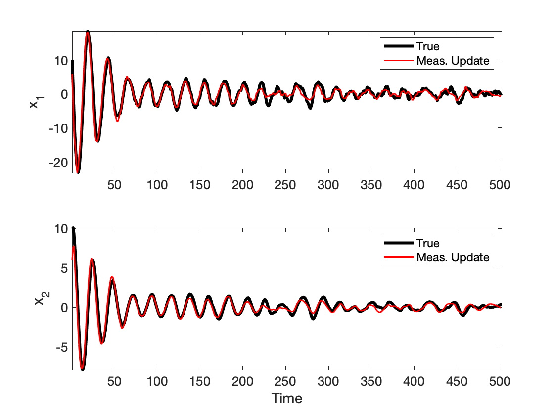
Figure VI-1. Estimates, $\hat{x}_{t\mid t}$, and the corresponding true vale of the state, $x_t$.
It is interesting to note that $\Sigma_{t+1\mid t}$ converges to a matrix $\Sigma_{\infty} = \lim_{t\to\infty}\Sigma_{t+1\mid t}$, which can be found by solving the discrete algebraic Riccati equation (DARE)
$$\Sigma_{\infty} {}={} A \Sigma_{\infty} A^\intercal {}+{} A \Sigma_{\infty}C^\intercal (C \Sigma_{\infty}C^\intercal + R)^{-1} C \Sigma_{\infty} A^\intercal {}+{} Q$$
In this example, we have
$$\Sigma_{\infty} {}={} \begin{bmatrix}1.0667 & 0.0894\\ 0.0894 & 0.1066\end{bmatrix}.$$
Sensor with bias
Now assume that the sensor gives us measurements with a constant or slowly varying bias, that is, the system output is
$$y_t = Cx_t + b_t + v_t,$$
where $b_t$ is a bias term, which we can model as
$$b_{t+1} = b_t + w^b_t,$$
where $w^b_t$ is an additive noise term, the process $(w^b_t)_t$ is iid zero-mean Gaussian with variance $Q^b$, and $w^b_t$ is independent of $x_t$.
We can then define the new state variable $z_t = (x_t, b_t)$ and attempt to estimate this news state, that is, to estimate $x_t$ and the measurement bias, $b_t$. The system dynamics and output can be written as
$$\begin{aligned} z_{t+1} =& \begin{bmatrix} A \\ & I \end{bmatrix}z_t + \tilde{w}_t, \\ y_{t} =& \begin{bmatrix} C & I \end{bmatrix}z_t + v_t, \end{aligned}$$
where $\tilde{w}_t = (w_t, w^b_t) \sim \mathcal{N}(0, \tilde{Q})$ with
$$\tilde{Q} = \begin{bmatrix}Q \\ & Q^b\end{bmatrix}.$$
More concisely, we have the system$$\begin{aligned} z_{t+1} =& \tilde{A}z_t + \tilde{w}_t, \\ y_{t} =& \tilde{C}z_t + v_t, \end{aligned}$$
with
$$\tilde{A} = \begin{bmatrix} A \\ & I \end{bmatrix}, \tilde{C} = \begin{bmatrix} C & I \end{bmatrix}.$$
We can now apply the Kalman filter to this system to estimate $z_t$.
You can experiment with this example on Google Colab.
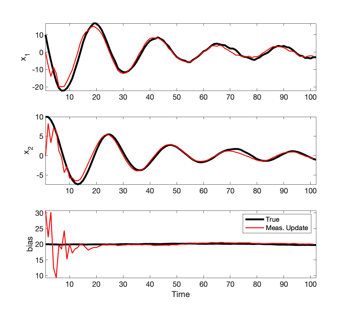
Figure VI-2. The Kalman filter is used to estiamate the states of the system and the bias on the sensor.
The reader can verify that the pair $(\tilde{A}, \tilde{C})$ is observable, and that $\Sigma_{\infty}$ exists and is finite. As an exercise, you can solve DARE to determine $\Sigma_{\infty}$ and verify that the sequence $\Sigma_{t+1\mid t}$ converges to $\Sigma_{\infty}$.
System dynamics with bias
Now consider a case where a constant term is acting on the system dynamics. In fact, let us consider the above system with an unknown constant term, $c_t\in{\rm I\!R}$, acting on the first coordinate of $x_t$, that is
$$x_{t+1} = \begin{bmatrix}0.98& -0.7 \\ 0.1& 0.9\end{bmatrix}x_t + \begin{bmatrix}c_t \\ 0\end{bmatrix} + w_t.$$
Suppose that $c_t$ is constant-ish; it is
$$c_{t+1} = c_t + w^c_t,$$
where $w^c_t$ is an iid normally distributed process, and it is independent of $x_t$. We can rewrite the above equations as
$$\begin{bmatrix}x_{t+1} \\ c_{t+1}\end{bmatrix} = \begin{bmatrix}0.98& -0.7 & 1\\ 0.1& 0.9 & 0 \\ 0 & 0 & 1\end{bmatrix} \begin{bmatrix}x_{t} \\ c_{t}\end{bmatrix} + \begin{bmatrix}w_{t} \\ w^c_{t}\end{bmatrix}.$$
Define $z_t=(x_t,c_t)$ and $\tilde{w}_t =(w_t, w^c_t)$. The output equation is
$$y_t = \begin{bmatrix}1 & 1 & 0\end{bmatrix}z_t + v_t.$$
We can then apply the Kalman filter to estimate $z_t$. The results are shown below in Figure VI-3
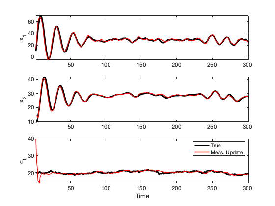
Figure VI-3. Here, the Kalman filter is used to estiamate the states of the system and the drift, $c_t$.
System with input
The Kalman filter can be applied to systems with inputs and often one needs to design a Kalman filter for a control system. There are, however, other cases of systems with inputs that are not control systems such as ones that we encounter in the study of attitude estimation.
Perfect knowledge of the input
Consider now a system with an input, $u_t$, which can be measured without error.
$$\begin{aligned}x_{t+1} {}={}& Ax_t + Bu_t + w_t,\\y_t {}={}& Cx_t + v_t.\end{aligned}$$
The input $u_t$ may depend on the state of the system (if often does), but does not depend on $w_t$. It is not difficult to generalise the update equations as follows:
$$\begin{aligned} \text{M/U} & \left[ \begin{array}{l} \hat{x}_{t{}\mid{}t} {}={} \hat{x}_{t{}\mid{}t-1} {}+{} \Sigma_{t{}\mid{}t-1}C^\intercal (C\Sigma_{t{}\mid{}t-1}C^\intercal + R)^{-1}(y_t - C\hat{x}_{t{}\mid{}t-1}) \\ \Sigma_{t{}\mid{}t} {}={} \Sigma_{t{}\mid{}t-1} {}-{} \Sigma_{t{}\mid{}t-1}C^\intercal (C\Sigma_{t{}\mid{}t-1}C^\intercal + R)^{-1} C\Sigma_{t{}\mid{}t-1} \end{array} \right. \\ \text{T/U} & \left[ \begin{array}{l} \hat{x}_{t+1{}\mid{}t} {}={} A \hat{x}_{t{}\mid{}t} + Bu_{t} \\ \Sigma_{t+1{}\mid{}t} {}={} A \Sigma_{t{}\mid{}t} A^\intercal + Q^\intercal \end{array} \right. \\ \text{Init.} & \left[ \begin{array}{l} \hat{x}_{0{}\mid{}-1} {}={} \tilde{x}_0 \\ \Sigma_{0{}\mid{}-1} {}={} P_0 \end{array} \right. \end{aligned}$$
Results are shown in Figure VI-4.
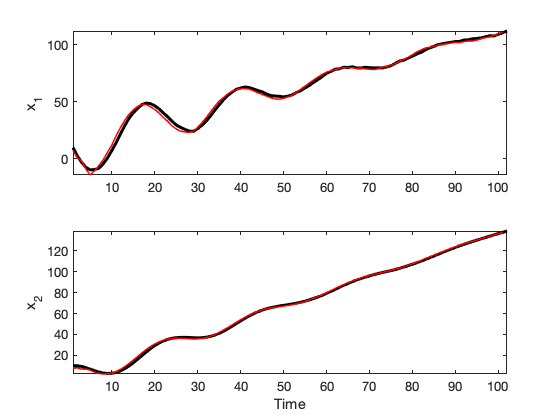
Figure VI-4. The Kalman filter is used to estiamate the states of the system with an input signal. Here we have used the same system matrices $A$ and $C$ as above, $B=[1 ~~ 0.04]^\intercal$ and an input $u_t = t$.
Imperfect knowledge of the input
Now suppose that the true input, $u_t$, can be measured and, in particular, we can measure a signal $u^{\rm meas}_t = u_t + n_t,$ where $n_t$ is an iid zero-mean Gaussian noise, $n_t\sim\mathcal{N}(0, N)$. Then, the system becomes
$$\begin{aligned}x_{t+1} {}={}& Ax_t + B(u^{\rm meas}_t - n_t) + w_t,\\y_t {}={}& Cx_t + v_t.\end{aligned}$$
which is in the form discussed above. We can rewrite this as
$$\begin{aligned} x_{t+1} {}={}& Ax_t + Bu^{\rm meas}_t - Bn_t + w_t \\ =& Ax_t + Bu^{\rm meas}_t + \begin{bmatrix}-B & I\end{bmatrix}\begin{bmatrix}n_t\\w_t\end{bmatrix}, \\ y_t {}={}& Cx_t + v_t.\end{aligned}$$
We can now define the new noise term $\tilde{w}_t = (n_t, w_t)$ and the matrix $G = [-B ~ I]$ and write
$$\begin{aligned} x_{t+1} {}={}& Ax_t + Bu^{\rm meas}_t + G\tilde{w}_t, \\ y_t {}={}& Cx_t + v_t,\end{aligned}$$
where
$$\tilde{w}_t\sim\mathcal{N}\left(0, \begin{bmatrix}N\\&Q\end{bmatrix}\right)$$
The Kalman filter update equations become
$$\begin{aligned} \text{M/U} & \left[ \begin{array}{l} \hat{x}_{t{}\mid{}t} {}={} \hat{x}_{t{}\mid{}t-1} {}+{} \Sigma_{t{}\mid{}t-1}C^\intercal (C\Sigma_{t{}\mid{}t-1}C^\intercal + R)^{-1}(y_t - C\hat{x}_{t{}\mid{}t-1}) \\ \Sigma_{t{}\mid{}t} {}={} \Sigma_{t{}\mid{}t-1} {}-{} \Sigma_{t{}\mid{}t-1}C^\intercal (C\Sigma_{t{}\mid{}t-1}C^\intercal + R)^{-1} C\Sigma_{t{}\mid{}t-1} \end{array} \right. \\ \text{T/U} & \left[ \begin{array}{l} \hat{x}_{t+1{}\mid{}t} {}={} A \hat{x}_{t{}\mid{}t} + Bu_{t}^{\rm meas} \\ \Sigma_{t+1{}\mid{}t} {}={} A \Sigma_{t{}\mid{}t} A^\intercal + BNB^\intercal + Q \end{array} \right. \\ \text{Init.} & \left[ \begin{array}{l} \hat{x}_{0{}\mid{}-1} {}={} \tilde{x}_0 \\ \Sigma_{0{}\mid{}-1} {}={} P_0 \end{array} \right. \end{aligned}$$
Results are shown in Figure VI-5.
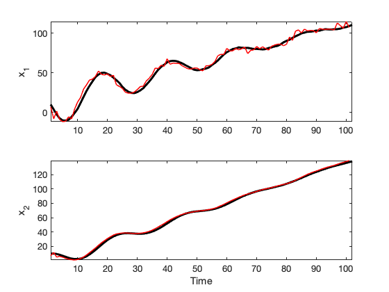
Figure VI-5. The Kalman filter is used to estiamate the states of the system with an input signal. Here we have used the same system matrices $A$ and $C$ as above, $B=[1 ~~ 0.04]^\intercal$ and an input $u_t = t$.
Read next: Kalman Filter VII: Recursive maximum a posteriori