Next post: Reading Vershynin’s HDP II: Subgaussianity
These are my notes on Ronan Vershynin's "High dimensional probability", Chapters 1 and 2 [1] and some solved exercises. Many of the results below focus on Bernoulli random variables.
Preliminaries
Exercise 1.1.3. Let \(X_1, X_2, \ldots\) be a sequence of iid random variables with mean \(\mu\) and a finite variance. Show that
$${\rm I\!E}\left|\frac{1}{N}\sum_{i=1}^{N}X_i - \mu\right| {}={} O\left(\frac{1}{\sqrt{N}}\right).$$
Solution. Without loss of generality we shall assume that $\mu=0$.
Firstly, we will get rid of that annoying absolute value as follows: Let us define
$$\bar{X}_N = \frac{1}{N}\sum_{i=1}^{N}X_i.$$
Then,
$${\rm I\!E}|\bar{X}_N| = {\rm I\!E} \sqrt{\bar{X}_N^2} \leq \sqrt{{\rm I\!E}[\bar{X}_N^2]},$$
where we used Jensen's inequality (using the fact that the square root is a concave function).
Now for ${\rm I\!E}[\bar{X}_N^2]$ we have
$${\rm I\!E}[\bar{X}_N^2] = \frac{1}{N^2} {\rm I\!E}\left(\sum_{i=1}^{N}X_i\right)^2 = \frac{1}{N^2} {\rm I\!E}\left[\sum_{i=1}^{N}X_i^2\right] =\frac{1}{N^2} N\sigma^2 = \frac{\sigma^2}{N}.$$
In the second equality we used the assumption of independence.
As a result
$${\rm I\!E}\left|\frac{1}{N}\sum_{i=1}^{N}X_i\right| {}\leq{} \sqrt{{\rm I\!E}[\bar{X}_N^2]} = \frac{\sigma}{\sqrt{N}}.$$
This completes the proof. $\Box$
Let us juxtapose the above result to the classical Lindeberg-Lévy central limit theorem (CLT):
Theorem 1 (Lindeberg-Lévy CLT). Let \(X_1, X_2, \ldots\) be a sequence of iid random variables with mean \(\mu\) and a finite variance \(\sigma^2\). Define $S_N = \sum_{i=1}^{N}X_i$ and
$$Z_N = \frac{S_N - {\rm I\!E[S_N]}}{\sqrt{{\rm Var}[S_N]}} = \frac{1}{\sigma\sqrt{N}}\sum_{i=1}^{N}(X_i - \mu).$$
Then, as \(N\to\infty\)
$$Z_N \overset{d}{\to} N(0, 1),$$
where \(\overset{d}{\to}\) means "convergence in distribution."
Proof. See [2].
We see that the Lindeberg-Lévy CLT also gives a \(1/\sqrt{N}\) type convergence result, but in the sense of convergence in distribution and it also gives us that "limit distribution", which is a normal.
Tails of the normal distribution
Exercise 2.1.4. (Truncated normal distribution) Let \(g\sim\mathcal{N}(0,1)\). Show that for all $t\geq 1$, we have
$$\begin{aligned}{\rm I\!E}[g^2 1_{g>t}] ={}& t \tfrac{1}{\sqrt{2\pi}}e^{-\tfrac{t^2}{2}} + {\rm P}[g > t] \\ \leq{}& \left(t+\tfrac{1}{t}\right)\tfrac{1}{\sqrt{2\pi}} e^{-\tfrac{t^2}{2}}.\end{aligned}$$
Solution. We have
$$\begin{aligned}{\rm I\!E}[g^2 1_{g>t}] ={}& \int_t^\infty x^2 e^{-\tfrac{x^2}{2}}\tfrac{1}{\sqrt{2\pi}} {\rm d}x \\ {}={}& \tfrac{1}{\sqrt{2\pi}} \int_t^\infty x^2 e^{-\tfrac{x^2}{2}} {\rm d}x \\ {}={}& \tfrac{1}{\sqrt{2\pi}} \int_t^\infty - x \left(e^{-\tfrac{x^2}{2}}\right)' {\rm d}x \\ {}={}& -\tfrac{1}{\sqrt{2\pi}} \left[ \left.x e^{-\tfrac{x^2}{2}}\right|_{t}^{\infty} - \int_t^\infty e^{-\tfrac{x^2}{2}} {\rm d}x\right] \\ {}={}& -\tfrac{1}{\sqrt{2\pi}} \left[ -te^{-\tfrac{t^2}{2}} - \int_t^\infty e^{-\tfrac{x^2}{2}}{\rm d}x\right] \\ {}={}& \tfrac{1}{\sqrt{2\pi}} te^{-\tfrac{t^2}{2}} + {\rm P}[g > t] \end{aligned}$$
We now invoke Proposition 2.1.2 in [1] according to which
$${\rm P}[g > t] \leq \tfrac{1}{t} \tfrac{1}{\sqrt{2\pi}} e^{-\tfrac{t^2}{2}}.$$
This completes the proof. $\Box$
A quick brush-up on probability inequalities
Let us start with Markov's inequality, which is one of the most fundamental probability inequalities. Many other well-known inequalities are derived from this.
Theorem 2 (Markov's inequality). Let \(X\) be a nonnegative random variable and \(t>0\). Then
$${\rm P}[X \geq t] \leq \frac{{\rm I\!E[X]}}{t}.$$
Chebyshev's inequality is a corollary of Markov's inequality.
Corollary 3 (Chebyshev's inequality). Let \(X\) be a random variable with mean $\mu$ and variance $\sigma^2$ and \(t>0\). Then
$${\rm P}[|X-\mu| \geq t] \leq \frac{\sigma^2}{t^2}.$$
Proof. The left-hand side of Chebyshev's inequality is ${\rm P}[|X-\mu| \geq t] = {\rm P}[(X-\mu)^2 \geq t^2]$. The random variable $Y=(X-\mu)^2$ is nonnegative, so we can apply Markov's inequality:
$${\rm P}[(X-\mu)^2 \geq t^2] \leq \frac{{\rm I\!E}[(X-\mu)^2 ]}{t^2} = \frac{\sigma^2}{t^2}.$$
This completes the proof. $\Box$
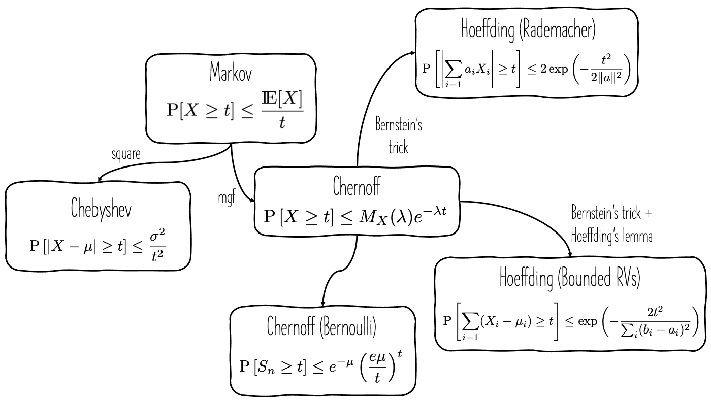
Figure 1. The Markov, Chebyshev, and Hoeffding inequalities.
Hoeffding’s inequality and more
Let us start by stating Hoeffding's inequality for independent symmetric Bernoulli random variables. Recall that the symmetric Bernoulli distribution - aka the Rademacher distribution - takes the values \(-\tfrac{1}{2}\) and \(\tfrac{1}{2}\) with equal probability.
Theorem 4 (Hoeffdings's inequality for symmetric Bernoulli). Let \(X_1, \ldots, X_N\) be independent symmetric Bernoulli random variables, and \(a{}\in{}{\rm I\!R}^N\). Then, for any \(t\geq 0\),
$${\rm P}\left[\sum_{i=1}^{N}a_i X_i \geq t\right] \leq \exp\left(- \frac{t^2}{2\|a\|_2^2}\right).\tag{H1}$$
Proof. The proof is given in [1], but a couple of things are left to the reader as an exercise.
Firstly, we assume without loss of generality that $\|a\|_2=1$. Let's see why: suppose we have proven (H1) with $\|a\|_2=1$, that is
$${\rm P}\left[\sum_{i=1}^{N}a_i X_i \geq t\right] \leq \exp\left(- \frac{t^2}{2}\right).\tag{\text{H1'}}$$
Then, if \(\|a\|\neq 1\) (and \(\|a\|\neq 0\)), we define $a_i' = a_i / \|a\|_2$ and we have
$${\rm P}\left[\sum_{i=1}^{N}a_i X_i \geq t\right] = {\rm P}\left[\sum_{i=1}^{N}\frac{a_i}{\|a\|_2} X_i \geq \frac{t}{\|a\|_2}\right] \overset{H1'}{\leq} \exp\left(- \frac{t^2}{2\|a\|_2^2}\right).$$
Now the trick is to use Markov's inequality after we apply the function $\exp(\lambda \cdot)$, where $\lambda > 0$, on both sides of the inequality inside the probability
$$\begin{aligned}{\rm P}\left[\sum_{i=1}^{N}a_i X_i \geq t\right] ={}& {\rm P}\left[\exp\left(\lambda\sum_{i=1}^{N}a_i X_i\right) \geq \exp(\lambda t)\right] \\ {}\leq{}& e^{-\lambda t} {\rm I\!E}\left[ \exp \left( \lambda \sum_{i=1}^{N}a_i X_i\right)\right].\end{aligned}$$
In the last step we applied Markov's inequality (Theorem 2). Next we have that
$$\begin{aligned}{\rm I\!E}\left[ \exp \left( \lambda \sum_{i=1}^{N}a_i X_i\right)\right] {}={}& {\rm I\!E}\left[ \prod_{i=1}^{N} \exp(\lambda a_i X_i)\right] \\ {}={}& \prod_{i=1}^{N} {\rm I\!E} \exp(\lambda a_i X_i)\end{aligned}$$
Then it is not difficult to see that ${\rm I\!E} \exp(\lambda a_i X_i) = \cosh(\lambda a_i).$ And here comes this exercise:
Exercise 2.2.3. (Bounding the hyperbolic cosine) Show that for all $x\in{\rm I\!R}$
$$\cosh (x) \leq \exp(x^2/2).$$
Solution. We want to prove that $\ln \cosh x \leq \tfrac{1}{2}x^2$. Define $f(x)=\ln \cosh x - \tfrac{1}{2}x^2$. Then $f'(x) = \tanh x - x$ and $f''(x) = -\tanh^2(x) \leq 0$, so $f$ is concave. The only solution of $f'(x)=0$ is $x=0$ and $f(0) = 0$, so $f$ has a maximum at $x=0$ and $f(x)\leq 0$ for all $x\in{\rm I\!R}$. $\Box$
Back to the proof of Hoeffding's inequality, we have
$$\begin{aligned}{\rm P}\left[\sum_{i=1}^{N}a_i X_i \geq t\right] {}\leq{}& e^{-\lambda t} \prod_{i=1}^{N} \exp(\lambda^2 a_i^2 / 2) \\ {}={}& \exp\left(-\lambda t + \tfrac{\lambda^2}{2}\sum_{i=1}^{N}a_i^2\right) \\ {}={}& \exp\left(-\lambda t + \tfrac{\lambda^2}{2}\right).\end{aligned}$$
Taking the minimum with respect to $\lambda > 0$, which is attained at $\lambda = t$, we prove Hoeffding's inequality. $\Box$
Remark. In the proof of the above version of Hoeffding's inequality we used the moment generating function (MGF) of a random variable $X$ which is defined as $M_X(\lambda) = {\rm I\!E}\exp(\lambda X)$. The MGF is a function that shows up all the time in such probability inequalities. The same argument as above is used to prove the Chernoff bound.
Hoeffding's inequality can be generalised to general bounded variables.
Theorem 5 (Hoeffdings's inequality for bounded random varibles). Let \(X_1, \ldots, X_N\) be independent random variables, bounded in $[m_i, M_i]$ for all $i$. Then, for any \(t > 0\),
$${\rm P}\left[\sum_{i=1}^{N} (X_i - {\rm I\!E}[X_i]) \geq t\right] \leq \exp\left(- \frac{2t^2}{\sum_{i=1}^{N}(M_i - m_i)^2}\right).\tag{H2}$$
Proof. See [3].
Exercise 2.2.8. (Boosting randomised algorithms) We have an algorithm for solving some decision problem, which makes a (binary) decision at random and returns the correct answer with probability \(\tfrac{1}{2}+\delta\), for some \(\delta > 0\), which is a little better than a random guess. We run the algorithm \(N\) times and take the majority vote. Show that for any \(\epsilon \in (0, 1)\), the answer is correct with probability \(1 - \epsilon\), as long as \(N \geq \tfrac{1}{2} \delta^{-2} \ln \epsilon^{-1}\).
Solution. Let $X_i$ be the outcome of the $i$-th run of the algorithm where $X_i=0$ corresponds to a correct decision, and $X_i$ corresponds to a wrong decision. Then ${\rm I\!E}[X_i] = \tfrac{1}{2}-\delta$ and $X_i$ is bounded in $[0, 1]$. By Hoeffding's inequality we see that
$$\begin{aligned}&{}{\rm P}\left[\sum_{i=1}^{N}(X_i - (\tfrac{1}{2}-\delta)) \geq t\right] \leq \exp\left(-\frac{2t^2}{N}\right) \\ \Leftrightarrow & {\rm P}\left[\sum_{i=1}^{N}X_i - N(\tfrac{1}{2}-\delta) \geq t\right] \leq \exp\left(-\frac{2t^2}{N}\right).\end{aligned}$$
The probability of the randomised algorithm (based on majority vote) to give the wrong answer is
$$\begin{aligned}P_{\rm err} ={}& {\rm P}\left[\sum_{i=1}^{N}X_i \geq \frac{N}{2}\right] \\ {}={}& \left[\sum_{i=1}^{N}X_i - N(\tfrac{1}{2}-\delta) \geq \frac{N}{2}- N(\tfrac{1}{2}-\delta)\right] \\ {}={}& \left[\sum_{i=1}^{N}X_i - N(\tfrac{1}{2}-\delta) \geq N\delta\right] \\ {}\leq{}& \exp\left(-\frac{2}{N}N^2\delta^2\right) = \exp(-2N\delta^2).\end{aligned}$$
To have $P_{\rm err} \leq \epsilon$ it suffices that
$$\exp(-2\delta^2 N) \leq \epsilon \Leftrightarrow N \geq \frac{1}{2\delta^2}\ln \tfrac{1}{\epsilon}.$$
This proves the assertion. $\Box$
Exercise 2.2.10. (Small ball probabilities) Let \(X_1, \ldots, X_N\) be nonnegative independent continuous random variables. Suppose that the pdf of $X_i$ are uniformly bounded by $1$. Then
- Show that ${\rm I\!E}[-tX_i] \leq 1/t$ for all $t > 0$
- Deduce that
$${\rm P}\left[\frac{1}{N}\sum_{i=1}^{N}X_i \leq \epsilon\right] \leq (e\epsilon)^N.$$
Solution. (1): Using the law of the unconscious statistician,
$${\rm I\!E}[e^{-tX_i}] = \int_{0}^{\infty} e^{-tx}p_{X_i}(x){\rm d}x \leq \int_0^\infty e^{-tx}{\rm d}x = \tfrac{1}{t}.$$
(2): We have
$$\begin{aligned} {\rm P}\left[\frac{1}{N}\sum_{i=1}^{N}X_i \leq \epsilon\right] {}={}& {\rm P}\left[\sum_{i=1}^{N}-\frac{X_i}{\epsilon} \leq -N\right] \\ {}\overset{\text{Ber.}}{=}{}& {\rm P}\left[\exp \left(\lambda \sum_{i=1}^{N}-\frac{X_i}{\epsilon}\right) \leq \exp(-\lambda N)\right] \\ {}\overset{\text{Mar.}}{\leq}{}& e^{\lambda N} {\rm I\!E}\left[ \exp\left(-\lambda \sum_{i=1}^{N}\frac{X_i}{\epsilon}\right)\right] \\ {}\overset{\text{Ind.}}{=}{}& e^{\lambda N} \prod_{i=1}^{N} {\rm I\!E} [-\lambda X_i / \epsilon] \leq e^{\lambda N}(\epsilon/\lambda)^N. \end{aligned}$$
Above, "Ber." stands for Bernstein's trick, "Mar." stands for Markov inequality, and "Ind." refers to the independence of $X_i$. The above inequality holds for $\lambda=1$, and the assertion follows. $\Box$
Chernoff bound for Bernoulli random variables
Hoeffding's inequality can be loose when the distribution is very skewed (e.g., Bernoulli with a very small value $p_i$). Chernoff's bound is a result that is more sensitive to the distribution of $X_i$. Let us state the result.
Theorem 6 (Chernoff's inequality). Let \(X_1, \ldots, X_N\) be independent Bernoulli random variables with parameters $p_i$. Define $S_N = \sum_{i=1}^{N}X_i$ and $\mu = {\rm I\!E}S_N$. Then, for any \(t > \mu\),
$${\rm P}\left[S_N \geq t\right] \leq e^{-\mu}\left( \frac{e\mu}{t}\right)^t.$$
We follow the same procedure as in the proof of Hoeffding's inequality:
$$\begin{aligned} {\rm P}[S_N \geq t] {}={}& {\rm P}[ \exp(\lambda S_N) \geq \exp(\lambda t)] \\ {}\leq{}& {\rm I\!E}\exp(\lambda S_N) \exp(-lambda t) \\ {}={} \prod_{i=1}^{N} {\rm I\!E} e^{\lambda X_i} / e^{\lambda t} \end{aligned}$$
We now use the fact that $X_i \sim {\rm Ber}(p_i)$. The mgf of $X_i$ is
$$\begin{aligned} {\rm I\!E} e^{\lambda X_i} {}={}& e^{\lambda}p_i + 1-p_i \\ {}={}& 1 + p_i(e^\lambda - 1) \\ {}\leq{}& \exp[p_i(e^{\lambda} - 1)], \end{aligned}$$
where we used the fact that $1+x \leq e^x$ for all $x\in{\rm I!R}$. Therefore,
$$\begin{aligned} &\prod {\rm I\!E} e^{\lambda X_i} {}\leq{} \exp\left[(e^\lambda - 1)\sum_{i=1}^{N}p_i\right] = \exp((e^\lambda - 1)\mu) \\ \Rightarrow & {\rm P}[S_N \geq t] \leq e^{-\lambda t} \exp[(e^\lambda - 1)\mu], \end{aligned}$$
for all $\lambda > 0$. We substitute $\lambda = \ln(t/\mu)$, which is positive because $t>\mu$, so
$${\rm P}[S_N] \leq e^{-\mu}\left(\frac{e\mu}{t}\right)^t.$$
This completes the proof. $\Box$
Let us recall the definition of the Poisson distribution.
Definition 7 (Poisson distribution). A random variable $X$ follows the Poisson distribution with parameter $\lambda>0$ - we denote $X\sim{\rm Poisson}(\lambda)$ - if it is supported on ${\rm I\!N}$ with pmf
$${\rm P}[X = k] = \frac{\lambda^k e^{-\lambda}}{k!}.$$
If $X\sim{\rm Poisson}(\lambda)$, then ${\rm I\!E}[X] = \lambda$ and ${\rm Var}[X] = \lambda$. The mgf of $X$ is
$${\rm I\!E}[\exp(sX)] = \exp[\lambda(e^s - 1)].$$
Exercise 2.3.3. Let $X\sim{\rm Poisson}(\lambda)$. Show that for all $t>\lambda$ we have
$${\rm P}[X \geq t] \leq e^{-\lambda} \left(\frac{e\lambda}{t}\right)^t.$$
Solution. We have
$$\begin{aligned} {\rm P}[X \geq t] {}={}& {\rm P}[\exp(sX) \geq \exp(st)] \\ {}={}& e^{-st}{\rm I\!E}[sX] \\ {}={}& e^{-st} e^{\lambda(e^s-1)}. \end{aligned}$$
Taking $s=\ln\tfrac{t}{\lambda}$ completes the proof. $\Box$
Exercise 2.3.8. (Normal approximation to Poisson) Let $X\sim{\rm Poisson}(\lambda)$. Show that as $\lambda\to\infty$ we have
$$\frac{X-\lambda}{\sqrt{\lambda}} \overset{d}{\to} \mathcal{N}(0, 1).$$
Solution. One way to show this is by using the following continuity theorem
Theorem 8 (Continuity theorem). Let $(X_n)_n$ be a sequence of random variables with cdf $F_n$ and corresponding mgf $M_{X_n}$. Let $X$ be a random variable with cdf $F$ and mgf $M_{X}$. If
$$M_{X_n} \to M_X,$$
pointwise over an open interval containing zero, then
$$F_n{}\to{}F,$$
at all points of continuity of $F$, that is $X_n \overset{d}{\to} X$.
Take a sequence of $\lambda_n > 0$ that goes to $\infty$. The mgf of $Z_n = \frac{X_n-\lambda_n}{\sqrt{\lambda_n}}$, where $X_n\sim{\rm Poisson}(\lambda_n)$ is
$$\begin{aligned} M_{Z_n}(t) {}={}& {\rm I\!E}\exp(tZ_n) = {\rm I\!E} \exp\left(t \frac{X_n - \lambda_n}{\sqrt{\lambda_n}}\right) \\ {}={}& {\rm I\!E}\exp\left(\frac{t X_n}{\sqrt{\lambda_n}} - \frac{t\lambda_n}{\sqrt{\lambda_n}}\right) \\ {}={}& \exp\left(-\frac{t\lambda_n}{\sqrt{\lambda_n}}\right) \exp\left[ \lambda_n \left( \exp\left(\frac{t}{\sqrt{\lambda_n}}\right) - 1 \right) \right] \\ {}={}& \exp \left[ -\frac{t\lambda_n}{\sqrt{\lambda_n}} + \lambda_n \left( \exp\frac{t}{\sqrt{\lambda_n}} - 1 \right) \right] \\ {}={}& \exp \left[ -\lambda_n \left(\frac{t}{\sqrt{\lambda_n}} + 1\right) + \lambda_n e^{t/\sqrt{\lambda_n}}\right] \end{aligned}$$
and we can see that as $n\to\infty$,
$$M_{Z_n}(t) \to \exp(t^2/2).$$
for all $t\in{\rm I\!R}$. This completes the proof. $\Box$
Note. Let us invoke the Lindeberg-Lévy central limit theorem. Take $Y_i{}\sim{}{\rm Poisson(1)}$, and $X_n = \sum_{i=1}^{n} Y_i \sim {\rm Poisson}(n)$, ${\rm I\!E}[X_n] = n$ and ${\rm Var}[X_n] = n$. From the Lindeberg-Lévy central limit theorem,
$$\frac{X_n-n}{\sqrt{n}} \overset{d}{\to} \mathcal{N}(0, 1).$$
This is a more concise way to solve Exercise 2.3.8.
References
- R. Vershynin, High Dimensional Probabiltiy: an introduction with applications in data science, Cambridge University Press, 2019
- F.W. Scholz, Central Limit Theorems and Proofs, Lecture Notes, Math/Stat 394, University of Washington, Winter 2019 (pdf)
- John Duchi, CS229 Supplemental Lecture notes: Hoeffding's inequality, Lecture Notes, CS229, Stanford (pdf)