Read first: The Kalman Filter VII: Recursive maximum a posteriori
Previous post: Beyond the Kalman Filter I: Extended Kalman Filter
In a previous post we saw that the Kalman filter is a recursive maximum a posteriori estimator and we formulated the full information estimation problem, which is an optimisation problem (very similar to a standard optimal control problem) which can be solved numerically, e.g., using OpEn.
Here we will repeat the same procedure, but we will lift the linearity and normality assumptions. In doing so, we will realise that we didn't need them in the first place. We will also introduce constraints on the states and inputs. However, we will not be able to come up with a recursive formula (moving horizon estimation amounts to solving an optimisation problem every time a new measurement is obtained).
Full information estimation
Consider the nonlinear dynamical system
$$\begin{aligned} x_{t+1} {}={} & f(x_t, w_t), \\ y_t {}={} & h(x_t) + v_t, \end{aligned}$$
where $x_0$, $w_t$ and $v_t$ are temporally and mutually uncorrelated, $w_t$ and $v_t$ follow known distributions (not necessarily normal). Note that since $w\in W$, it is $p_w(w)=0$ for $w\notin W$.
$$\begin{aligned} p_{w_t}(w) {}\propto{} & \exp [-\ell_w(w)], \\ p_{v_t}(v) {}\propto{} & \exp [-\ell_v(v)], \\ p_{x_0}(x_0) {}\propto{} & \exp [-\ell_{x_0}(x_0)]. \end{aligned}$$
The disturbance terms can be constrained - in particular we assume that $w_t\in W$ and $v_t \in V$ (nonempty, closed), Constrained states: $x_t \in X$. The extended Kalman filter cannot take into account constraints.
In order to describe the constraints we assume that $\ell_w(w) {}={} \infty$, for $w\notin W$, $\ell_v(v) {}={}$ for $v\notin V$, and $\ell_{x_0}(x_0) {}={} \infty$, for $x_0\notin X$, therefore ${\rm dom} \ell_w = W$, ${\rm dom} \ell_v = V$, ${\rm dom} \ell_{x_0} = X$.
Our objective is to estimate $x_{0:T}=(x_0, \ldots, x_{T})$ and $w_{0:T-1}=(w_0, \ldots, w_{T-1})$ from measurements $y_{0:T-1}=(y_0, \ldots, y_{T-1})$ using a MAP approach. The posterior distribution is
$$p(x_{0:T}, w_{0:T-1} {}\mid{} y_{0:T-1}) {}\propto{} p(y_{0:T-1} {}\mid{} x_{0:T}, w_{0:T-1}) p(x_{0:T}, w_{0:T-1}).$$
We can show that
$$p(x_{0:T}, w_{0:T-1}) {}={} \begin{cases} 0, & \text{ if } x_{t+1}{}\neq{}f(x_t, w_t) \text{ or } x_{t+1} \notin X \\ p_{x_0}(x_0)\prod_{t=0}^{N-1}p_{w_t}(w_t), & \text{ otherwise} \end{cases}$$
This can be written as
$$p(x_{0:T}, w_{0:T-1}) {}={} p_{x_0}(x_0)\prod_{t=0}^{N-1}p_{w_t}(w_t) 1_{\{0\}}(x_{t+1}-f(x_t, w_t))1_{X}(x_{t+1}),$$
where $1_{A}(s) = 1$ if $s\in A$ and $1_{A}(s) = 0$ otherwise. Furthermore,
$$p(y_{0:T-1} {}\mid{} x_{0:T}, w_{0:T-1}) {}={} \prod_{t=0}^{T-1}p(y_t {}\mid{} x_t) {}={} \prod_{t=0}^{T-1}p_{v_t}(y_t - h(x_t)).$$
With the convention $-\ln 0 = \infty$, we have $-\ln 1_{A}(s) = \delta_{A}(s)$, define the function
$$\begin{aligned} L(x_{0:T}, w_{0:T-1} {}\mid{} y_{0:T-1}) {}={} & -\ln p(x_{0:T}, w_{0:T-1} {}\mid{} y_{0:T-1}) \\ {}={} & \ell_{x_0}(x_0) {}+{} \sum_{t=0}^{T-1}\ell_{w_t}(w_t) + \ell_{v_t}(y_t - h(x_t)) \\ & \qquad\qquad\qquad + \delta_{\{0\}}(x_{t+1}-f(x_t, w_t)) + \delta_X(x_{t+1}). \end{aligned}$$
The MAP estimate of $x_{0:T}$ and $w_{0:T-1}$ given $y_{0:T-1}$ can be determined by solving
$$\operatorname*{minimise}_{x_{0:T}, w_{0:T-1}}L(x_{0:T}, w_{0:T-1} {}\mid{} y_{0:T-1}),$$
which is equivalently written as
$$\begin{aligned} \mathbb{P}^{\rm map}_T(y_{0:T-1}){}:{} \operatorname*{minimise}_{x_{0:T}, w_{0:T-1}}\, & \ell_{x_0}(x_0) + \sum_{t=0}^{T-1}\ell_{w_t}(w_t) + \ell_{v_t}(y_t - h(x_t)), \\ \text{subject to: } & x_{t+1}=f(x_t, w_t),\, t\in{\rm I\!N}_{[0, T-1]}, \\ & x_{t}\in X,\, t\in{\rm I\!N}_{[0, T]}. \end{aligned}$$
At time $T$, having observed $y_{0:T-1}$ we can solve the above problem to estimate $x_{0:T}$ and $w_{0:T-1}$.
This problem can be solved explicitly if $f$ is linear and $w_t$, $v_t$ and $x_0$ are independent and normally distributed. However, as time goes on and we accumulate more measurements, the size of the optimisation problem grows unbounded. We will use (forward) DP to cast this problem as a fixed-horizon optimal control problem (a problem with horizon $N$ that does not grow).
Forward Dynamic Programming
Let us apply the forward dynamic programming procedure as we did in this post.
$$\begin{aligned} \widehat{V}_T^\star {}={} & \min_{{x_{0:T},w_{0:T-1}}} \left\{ \ell_{x_0}(x_0) {}+{} \sum_{t=0}^{T-1} \underbrace{\ell_{w_t}(w_t) + \ell_{v_t}(y_t - h(x_t))}_{\ell_t(x_t, w_t)} \left| \begin{array}{l} x_{t+1} = f(x_t, w_t), \\ t\in{\rm I\!N}_{[0, T-1]} \end{array} \right. \right\} \\ {}={} & \min_{{x_{0:T},w_{0:T-1}}} \left\{ \ell_{x_0}(x_0) + \sum_{t=0}^{T-1} {\ell_t(x_t, w_t)} \left| \begin{array}{l} x_{t+1} = f(x_t, w_t), \\ t\in{\rm I\!N}_{[0, T-1]} \end{array} \right. \right\} \\ {}={} & \min_{{x_{1:T},w_{1:T-1}}} \Bigg\{ \underbrace{ \min_{x_0, w_0} \left\{ \ell_{x_0}(x_0) + \ell_0(x_0, w_0) {}\mid{} x_1 = f(x_0, w_0) \right\} }_{V_1^{\star}(x_1)} \rule{0cm}{0.8cm} \\ & \hspace{6em} \rule{0cm}{0.8cm} {}+{} \sum_{t=1}^{T-1} \ell_t(x_t, w_t)\, \left| \begin{array}{l} x_{t+1} = f(x_t, w_t), \\ t\in{\rm I\!N}_{[1, T-1]} \end{array} \right. \Bigg\} \\ {}={} & \min_{{x_{1:T},w_{1:T-1}}} \left\{ {V_1^{\star}(x_1)} {}+{} \sum_{t=1}^{T-1} \ell_t(x_t, w_t) \left| \begin{array}{l} x_{t+1} = f(x_t, w_t), \\ t\in{\rm I\!N}_{[1, T-1]} \end{array} \right. \right\}, \end{aligned}$$
and we can keep applying this procedure forwards. The forward dynamic programming procedure can be written concisely as
$$\begin{aligned} V_0^\star(x_0) {}={} & \ell_{x_0}(x_0), \\ V_{t+1}^{\star}(x_{t+1}) {}={} & \min_{x_0, w_0} \left\{ V_t^\star(x_t) + \ell_t(x_t, w_t) {}\mid{} x_{t+1} = f(x_t, w_t) \right\}, \end{aligned}$$
and $\widehat{V}_T^\star {}={} \min_{x_{T}}V_T^\star(x_T)$. Note that $V_t^\star$ corresponds to $-\ln p(x_t {}\mid{} y_{0:t-1})$. This allows us to write the MAP estimation problem as
$$\begin{aligned} \operatorname*{minimise}_{x_{T-N:T}, w_{T-N:T-1}}\, & V_{T-N}^\star(x_{T-N}) {}+{} \sum_{t=T-N}^{T-1}\ell_{t}(x_t, w_t), \\ \text{subject to: } & x_{t+1}=f(x_t, w_t),\, t\in{\rm I\!N}_{[T-N, T-1]}, \\ & x_{t}\in X,\, t\in{\rm I\!N}_{[T-N, T]}. \end{aligned}$$
This problem uses a window of measurements of fixed length $N$. However, the arrival cost $V_{T-N}^\star$ is very difficult to compute.
Moving horizon estimation
... instead, we shall use a different prior weighting function $\Gamma_{T-N}(x)$ and solve
$$\begin{aligned} \mathbb{P}_{N}^{\rm mhe}:\operatorname*{minimise}_{x_{T-N:T}, w_{T-N:T-1}}\, & {\Gamma_{T-N}}(x_{T-N}) {}+{} \sum_{t=T-N}^{T-1}\ell_{t}(x_t, w_t), \\ \text{subject to: } & x_{t+1}=f(x_t, w_t),\, t\in{\rm I\!N}_{[T-N, T-1]}, \\ & x_{t}\in X,\, t\in{\rm I\!N}_{[T-N, T]}. \end{aligned}$$
One possible choice for the prior weighting is \(\Gamma_{T-N}(x) = 0\) which works well if $N$ is sufficiently large and some additional assumptions are satisfied.
The above problem is known as the moving horizon estimation problem. Similar to model predictive control, every time a new measurement is obtained, an optimisation problem is solved to estimate the $N+1$ latest states of the system.
Moving Horizon Estimation vs EKF
This example has been taken from [1].
Consider the following chemical reaction takes place in gaseous phase
$$2A {}\longrightarrow{} B,$$
with rate coefficient $k=0.16$ and reaction rate $r=kP_A^2$, where $P_A$ and $P_B$ are the partial pressures of $A$ and $B$ respectively. The state is the vector $x=[P_A ~ P_B]^\intercal$ and the system dynamics is
$$x_{t+1} = \underbrace{\begin{bmatrix} \frac{x_{t, 1}}{2k\Delta t x_{t, 1} + 1} \\ x_{t, 2} + \frac{k \Delta t x_{t, 1}^2}{2k\Delta t x_{t, 1} + 1} \end{bmatrix}}_{F(x_t)} + w_t,$$
where $\Delta t = 0.1$ is the sampling time. We can measure the total pressure, that is
$$y_t = \begin{bmatrix} 1 & 1 \end{bmatrix}x_t + v_t,$$
where $v_t\sim\mathcal{N}(0, 0.1^2)$ ($R=0.1^2$) and $w_t \sim \mathcal{N}(0, 0.001^2 I_2)$ ($Q=0.001^2 I_2$). Suppose that $x_0 = [3 ~ 1]^\intercal$ while our prior knowledge about $x_0$ is $\bar{x}_0 = [0.1 ~ 4.5]^\intercal$ and $P_0 = 6^2 I_2$.
In Figure 1 we see that EKF doesn't do a very good job in estimating the states. The EKF does not take into account the state constraints and it propagates the covariance matrices based on the local linearisation of the dynamics and the output equation.
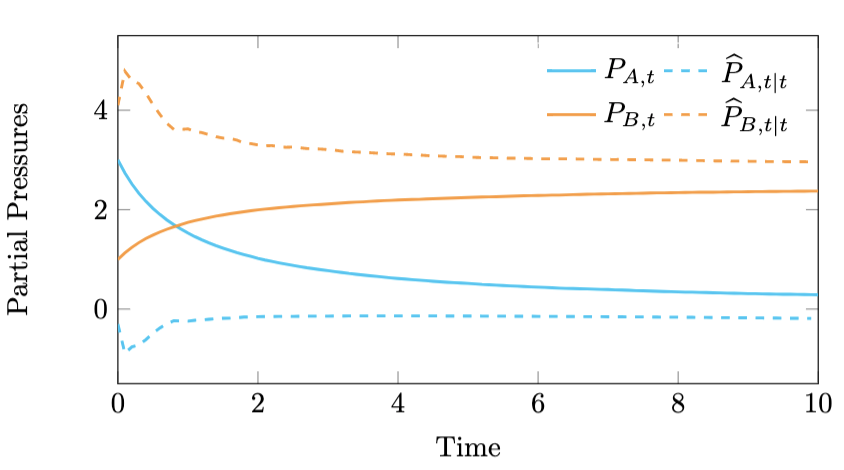
Figure 1. Failure of the extended Kalman filter.
We see that the EKF estimates are of rather poor quality and $\widehat{P}_{B, t\mid t}$ gives negative pressure values, which do not make sense.
Next, we formulate the following FIE-MHE problem that is solved at time $T-1$ using all measurements $y_{0:T-1}$
$$\begin{aligned} \mathbb{P}_{T}(y_{0:T-1}) {}:{} \operatorname*{minimise}_{x_{0:T}, w_{0:T-1}, v_{0:T-1}}\, & \tfrac{1}{2}\|x_0 - \bar{x}_0\|_{P_0^{-1}}^2 + \tfrac{1}{2}\sum_{t=0}^{T-1}\|w_t\|_{Q^{-1}}^2 + \|v_t\|_{R^{-1}}^2, \\ \text{subject to: } & x_{t+1}=F(x_t) + w_t,\, t\in{\rm I\!N}_{[0, T-1]}, \\ & y_t = [1 ~ 1]x_t + v_t, \, t\in{\rm I\!N}_{[0, T-1]}, \\ & x_{t} {}\geq{} 0,\, t\in{\rm I\!N}_{[0, T]}. \end{aligned}$$
In Figure 2 we see that the MHE estimates trace the trajectory of the actual system states.
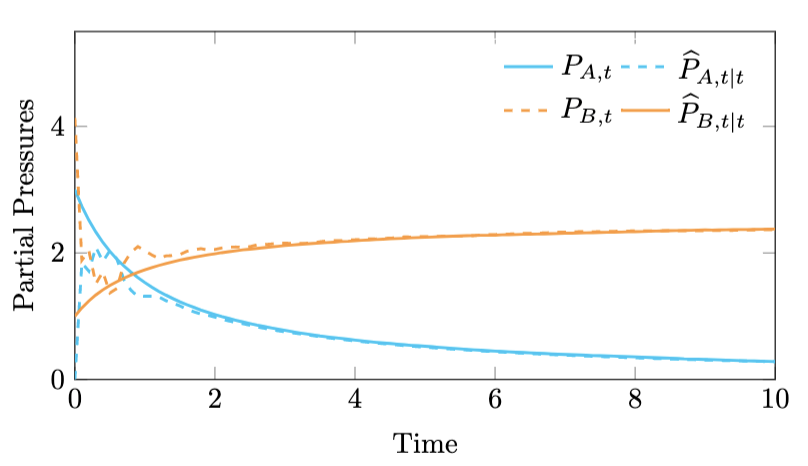
Figure 2. Moving horizon estimation produces high quality estimates.
References
[1] E.L. Haseltine & J.B. Rawlings, A Critical Evaluation of Extended Kalman Filtering and Moving Horizon Estimation, Ind. Eng. Chem. Res. 2005, 44(8):2451-60.
[2] John Bagter Jørgensen, Moving Horizon Estimation and Control, Technical University of Denmark, 2004 (PhD dissertation)
[3] F. Allgöwer, T. A. Badgwell, J. S. Qin, J. B. Rawlings & S. J. Wright, Nonlinear Predictive Control and Moving Horizon Estimation - An Introductory Overview, Advances in Control, 1999:391–449, Springer, London.
[4] Christopher V. Rao, Moving Horizon Strategies for the Constrained Monitoring and Control of Nonlinear Discrete-Time Systems, University of Winsconsin-Madison, 2000 (PhD dissertation)