Read first: Kalman Filter III: Measurement and time updates
Linearisation
Consider a function $f:{\rm I\!R}^n\to{\rm I\!R}^m$, which can be written as follows
$$f(x) {}={} \begin{bmatrix} f_1(x) \\ f_2(x) \\ \vdots \\ f_m(x) \end{bmatrix},$$
where $f_i:{\rm I\!R}^n\to{\rm I\!R}$ are smooth functions. The Jacobian matrix of $f$ is a function $Jf:{\rm I\!R}^n\to{\rm I\!R}^{m\times n}$ given by
$$Jf(x) = \begin{bmatrix} \nabla f_1(x)^\intercal \\ \nabla f_2(x)^\intercal \\ \vdots \\ \nabla f_m(x)^\intercal \end{bmatrix} {}={} \begin{bmatrix} \frac{\partial f_1}{\partial x_1} & \frac{\partial f_1}{\partial x_2} & \cdots & \frac{\partial f_1}{\partial x_n} \\ \frac{\partial f_2}{\partial x_1} & \frac{\partial f_2}{\partial x_2} & \cdots & \frac{\partial f_2}{\partial x_n} \\ \vdots & \vdots & \ddots & \vdots \\ \frac{\partial f_m}{\partial x_1} & \frac{\partial f_m}{\partial x_2} & \cdots & \frac{\partial f_m}{\partial x_n} \end{bmatrix}$$
Suppose that $f:{\rm I\!R}^n\to{\rm I\!R}^m$ is a differentiable function. Let $X$ be a ${\rm I\!R}^n$-valued random variable. Define $Y=f(X)$ and take $\overline{X} \coloneqq {\rm I\!E}[X]$, $\Sigma_X \coloneqq {\rm Var}[X]$. Then,
$$Y = f(X) \approx f(\overline{X}) + Jf(\overline{X})(X-\overline{X}),$$
so the expectation and variance of $Y$ can be approximated by
$$\begin{aligned} {\rm I\!E}[Y] {}\approx{} & \overline{Y}_{\rm lin} {}\coloneqq{} f(\overline{X}) \\ {\rm Var}[Y] {}\approx{} & \Sigma_{Y, {\rm lin}} {}\coloneqq{} Jf(\overline{X}) \Sigma_X Jf(\overline{X})^\intercal. \end{aligned}$$
Roughly speaking, this approximation is good when $f$ is not too nonlinear (in the sense that the higher-order terms of Taylor's theorem that we omitted can be ignored) and $\Sigma_X$ is not too large.
For example, consider the function $f(x)=e^x$ and $X{}\sim{}\mathcal{N}(\mu,\sigma^2)$. Then, the linearisation-based estimation of the expected value and variance of $Y=f(X)$ are
$$\begin{aligned} \overline{Y}_{\rm lin} {}={} & e^{\mu}, \\ \Sigma_{Y, {\rm lin}} {}={} & e^{2\mu} \sigma^2. \end{aligned}$$
It is known that
$$\begin{aligned} {\rm I\!E}[Y] {}={} & e^{\mu+\sigma^2/2}, \\ {\rm Var}[Y] {}={} & (e^{\sigma^2}-1)e^{2\mu+\sigma^2}. \end{aligned}$$
Note: If $X{}\sim{}\mathcal{N}(\mu, \sigma^2)$, then $Y=e^X$ follows the log-normal distribution with parameters $\mu$ and $\sigma$, which has a known pdf, mean and variance.
| ${\rm I\!E}[Y]$ | ${\rm Var}[Y]$ | ||
| $X{}\sim{}\mathcal{N}(0.5, 0.01)$ | Correct value | 1.6570 | 0.0276 |
| Linearisation | 1.6487 | 0.0272 | |
| $X{}\sim{}\mathcal{N}(0.5, 0.15)$ | Correct value | 2.1170 | 2.2237 |
| Linearisation | 1.6487 | 1.3591 |
Note that the linearisation works well when the variance is small. The linearisation method leads to the extended Kalman Filter.
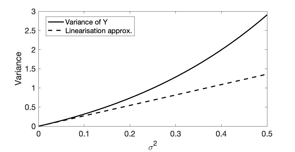
Figure 1. True value of the variance of $Y$ (solid line) and linearisation-based estimation (dashed line) for $\mu=0.5$.
It is becoming evident: the extended Kalman filter (which is based on the linearisation) will be far from being optimal and may even diverge. However, it often works decently well in practice. In any case, let us see how it works.
The Extended Kalman Filter
Consider the following nonlinear system
$$\begin{aligned} x_{t+1} {}={} & f(x_t, w_t), \\ y_t {}={} & h(x_t, v_t), \end{aligned}$$
where $x_0$, $(w_t)_t$ and $(v_t)_t$ are independent, $(w_t)_t$ and $(v_t)_t$ have zero mean and covariance matrices $Q_t$ and $R_t$ respectively. Even if $w$ and $v$ are Gaussian, $x_t$ and $y_t$ may not be (and typically are not).
The objective is to determine $\hat{x}_{t+1{}\mid{}t}$, $\hat{x}_{t{}\mid{}t}$ and the corresponding covariance matrices.
EKF uses the linearisation technique. It can work well, especially when variance is low or the system is approximately linear. It is a very popular in practice (especially in navigation). It is not an optimal estimator; may even diverge.
How it works: use the linearisation method to produce approximate measurement and time update steps.
For the measurement update step, we start with the standard initialisation: $\hat{x}_{0{}\mid{}-1}{}={}\tilde{x}_0$ and $\Sigma_{0{}\mid{}-1}{}={}P_0$ and we linearise the output function at $x=\hat{x}_{t{}\mid{}t-1}$:
$$\begin{aligned} C {}={} & J_x h(\hat{x}_{t{}\mid{}t-1}, 0), \\ \widetilde{R} {}={} & J_v h (\hat{x}_{t{}\mid{}t-1}, 0) \, R\, J_v h (\hat{x}_{t{}\mid{}t-1}, 0)^\intercal \end{aligned}$$
The measurement update is
$$\begin{aligned} \hat{x}_{t{}\mid{}t} {}={} & \hat{x}_{t{}\mid{}t-1} {}+{} \Sigma_{t{}\mid{}t-1}C^\intercal (C\Sigma_{t{}\mid{}t-1}C^\intercal + \widetilde{R})^{-1}(y_t - h(x_{t\mid t-1}, 0)) \\ \Sigma_{t{}\mid{}t} {}={} & \Sigma_{t{}\mid{}t-1} {}-{} \Sigma_{t{}\mid{}t-1}C^\intercal (C\Sigma_{t{}\mid{}t-1}C^\intercal + \widetilde{R})^{-1} C\Sigma_{t{}\mid{}t-1} \end{aligned}$$
Then, for the time update step, we linearise the dynamics at $x=\hat{x}_{t\mid t}$
$$\begin{aligned} A {}={} & J_x f(\hat{x}_{t{}\mid{}t}, 0), \\ \widetilde{Q} {}={} & J_w f(\hat{x}_{t{}\mid{}t}, 0) \, Q\, J_w f(\hat{x}_{t{}\mid{}t}, 0)^\intercal \end{aligned}$$
The time update is
$$\begin{aligned} \hat{x}_{t+1\mid t} {}={} & f(\hat{x}_{t\mid t}, 0), \\ \Sigma_{t+1 \mid t} {}={} & A\Sigma_{t \mid t}A^\intercal + \widetilde{Q}. \end{aligned}$$
Application of EKF to position estimation
Let $r_t,u_t,a_t\in{\rm I\!R}^2$ be the (planar) position, velocity and acceleration of a vehicle with dynamics
$$\begin{aligned} r_{t+1} {}={} & r_{t} + 0.2 u_t, \\ u_{t+1} {}={} & u_t + 0.2 a_t, \\ a_{t+1} {}={} & \Phi a_{t} + w_t, \end{aligned}$$
where $w_t \sim \mathcal{N}(0_2, 0.2I_2)$, and
$$\Phi {}={} \begin{bmatrix} \phantom{-}0.50 & 0.87 \\ -0.87 & 0.48 \end{bmatrix}.$$
Three beacons are positioned at $r^{(1)} = (3, 2)$, $r^{(2)}=(2, -3)$ and $r^{(3)}=(-5, 3)$; a sensor can measure the distances to these points - in particular $y_{i, t} {}={} \|r - r^{(i)}\|_2 + v_{i,t},\ i\in{\rm I\!N}_{[1,3]},$ where $v_{i,t} \sim \mathcal{N}(0, 4)$.
We have a system with state vector $\bm{x}_t = (r_t, u_t, a_t)$ and output $y_t$. The dynamics is linear
$$\bm{x}_{t+1} = \begin{bmatrix} I_2 & 0.2I_2\\ & I_2 & 0.2I_2 \\ & & \Phi \end{bmatrix} \bm{x}_{t} + \begin{bmatrix} 0_{4\times 2} \\ I_2 \end{bmatrix} w_t,$$
but the output equation is nonlinear
$$ y_t {}={} h(\bm{x}_t, v_t),$$
The gradient of $\|x\|$ is $\nabla \|x\| = x/\|x\|$, for $x\neq 0$. Let us denote this function by $\pi$. Then,
$$\begin{aligned} J_x h(x, v) {}={} & \begin{bmatrix} \begin{array}{c} \pi(r_t - r^{(1)})^\intercal \\ \pi(r_t - r^{(2)})^\intercal \\ \pi(r_t - r^{(3)})^\intercal \end{array} & 0_{3\times 4} \end{bmatrix}, \end{aligned}$$
and $J_v h(x, v){}={} I_3$.
Some simulation results are shown below. You can play with the Python code on Google Colab. Some simulation results are shown below.
Here is an example in Python. Let us start by defining the problem data
Phi = np.array([[0.5, 0.87], [-0.87, 0.48]])
anchors = np.array([[3, 2], [2, -3], [-5, -3]])
ny = len(anchors)
nx = 6
Q = np.array([[0.2, 0], [0, 0.2]])
R = 4*np.eye(ny)

A = np.block([[np.eye(2), 0.2*np.eye(2), np.zeros((2, 2))],
    [np.zeros((2, 2)), np.eye(2), 0.2*np.eye(2)],
    [np.zeros((2, 4)), Phi]])

Qbar = np.block([[np.zeros((4, 6))], [np.zeros((2, 4)), Q]])
Next, we need to define $f$, $h$ and $J_x h$
def f(x, w):
    """
    System dynamics, x+ = f(x, w)
    """
    r, u, a = x[:2], x[2:4], x[4:6]
    x_plus = np.concatenate((r + u / 5, u + a / 5, Phi @ a + w))
    return x_plus


def h(x, v):
    """
    Output relationship, y = h(x, v)
    """
    r = x[:2]
    y = np.empty(shape=(ny,))
    for i in range(ny):
        y[i] = np.linalg.norm(r - anchors[i]) + v[i]
    return y

def dh_x(x, _v):
    """
    Gradient of h wrt x
    """
    r = x[:2]
    dh = np.zeros(shape=(ny, nx))
    for i in range(ny):
        dh[i, :2] = (r-anchors[i]).T / np.linalg.norm(r-anchors[i])
    return dh
and here is an implementation of the extended Kalman filter
# Initialisation
x_t = np.array([-3, 1.5, 1, 0, 0, 0])
x_t_pred = np.array([0, 0, 0, 0, 0, 0])
sigma_t_pred = 100*np.eye(6)

N = 100

x_true_cache = np.zeros((N, 6))
x_meas_cache = np.zeros((N-1, 6))
x_true_cache[0, :] = x_t

for t in range(N-1):
    # obtain measurement
    v_t = np.random.multivariate_normal([0]*ny, R)
    y_t = h(x_t, v_t)

    # measurement update
    C = dh_x(x_t, 0)
    Z = C @ sigma_t_pred @ C.T + R
    x_t_meas = x_t_pred + sigma_t_pred @ C.T @ np.linalg.solve(Z, y_t-h(x_t_pred, [0]*ny))
    x_meas_cache[t, :] = x_t_meas
    sigma_t_meas = sigma_t_pred - sigma_t_pred @ C.T @ np.linalg.solve(Z, C @ sigma_t_pred)

    # Dynamics
    w_t = np.random.multivariate_normal([0, 0], Q)
    x_t = f(x_t, w_t)
    x_true_cache[t+1, :] = x_t

    # Time update
    x_t_pred = f(x_t_meas, [0, 0])
    sigma_t_pred = A @ sigma_t_meas @ A.T + Qbar
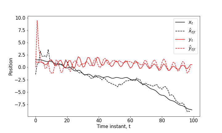
Figure 2. The $x$ and $y$ coordinates of the vehicle and the estimated positions (measurement updates) using the extended Kalman filter.
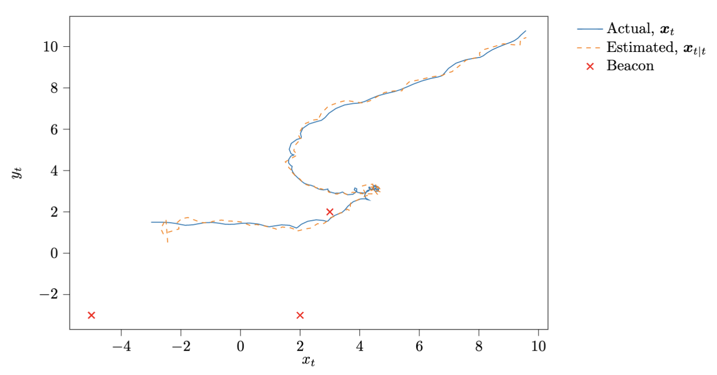
Figure 3. Another simulation showing the motion of the vehicle on the $(x, y)$ plane and the estimated trajectory.