Read first: Kalman Filter III: Measurement and time updates
Read next: Kalman Filter V: It’s BLUE!
Problem statement
Consider a vehicle that can only move on a straight line (e.g., a train). The initial position, $x_0$, of a vehicle is inexactly known. Suppose that $x_0 \sim \mathcal{N}(0, 100).$ The velocity of the vehicle, $u_t$, is approximately $10\, {\rm m}/{\rm s}$ in the sense $u_t \sim \mathcal{N}(10, 8).$ The position of the vehicle can be measured using a GPS system every $h=0.05\, {\rm s}$ using a sensor with additive noise $v_t\sim\mathcal{N}(0, 15)$.
The dynamics of the position of the vehicle is
$$\begin{aligned} x_{t+1} {}={} & x_t + hu_t, \\ y_t {}={} & x_t + v_t. \end{aligned}$$
However, $u_t$ is not a zero-mean random variable! However, note that the velocity can be written as $u_t = \bar{u}_t + w_t,$ where $\bar{u}_t = 10 \, {\rm m}/{\rm s}$ and $w_t \sim \mathcal{N}(0, 8)$. Since $\bar{u}_t$ is constant, $\bar{u}_{t+1} = \bar{u}_t$, so
$$ \begin{bmatrix} x_{t+1} \\ \bar{u}_{t+1} \end{bmatrix} {}={} \underbrace{ \begin{bmatrix} 1 & h \\ 0 & 1 \end{bmatrix} }_{A} \underbrace{ \begin{bmatrix} x_{t} \\ \bar{u}_{t} \end{bmatrix} }_{\bm{x}_t} + \underbrace{ \begin{bmatrix} h \\0 \end{bmatrix} }_{G} w_t.$$
The state of the system is $\bm{x}_t = (x_t, \bar{u}_t)$ with
$$\bm{x}_0 \sim \mathcal{N}\left(\begin{bmatrix}0\\10\end{bmatrix},\begin{bmatrix}100 & 0\\0 & 0\end{bmatrix}\right).$$
The output of the system is $y_t = [1 {}~{} 0]\,\bm{x}_t + v_t.$ Overall, the system is in the form of
$$\begin{aligned}x_{t+1} {}={} & A_t x_t + G_t w_t,\\y_t {}={} & C_t x_t + v_t,\tag{S}\end{aligned}$$
where
$$\begin{aligned} A = \begin{bmatrix}1 & h\\0 & 1\end{bmatrix}, G = \begin{bmatrix}h\\0\end{bmatrix}, C = \begin{bmatrix}1 & 0\end{bmatrix}, P_0 = \begin{bmatrix}100 & 0\\0 & 0\end{bmatrix}, Q = 8, R = 15, \end{aligned}$$
and $\bar{\bm{x}}_0 = (\tilde{x}_0, \tilde{\bar{u}}_0) = (0,10)$.
The true and estimated trajectories of the vehicle are shown below in Figures IV.1 and IV.2.
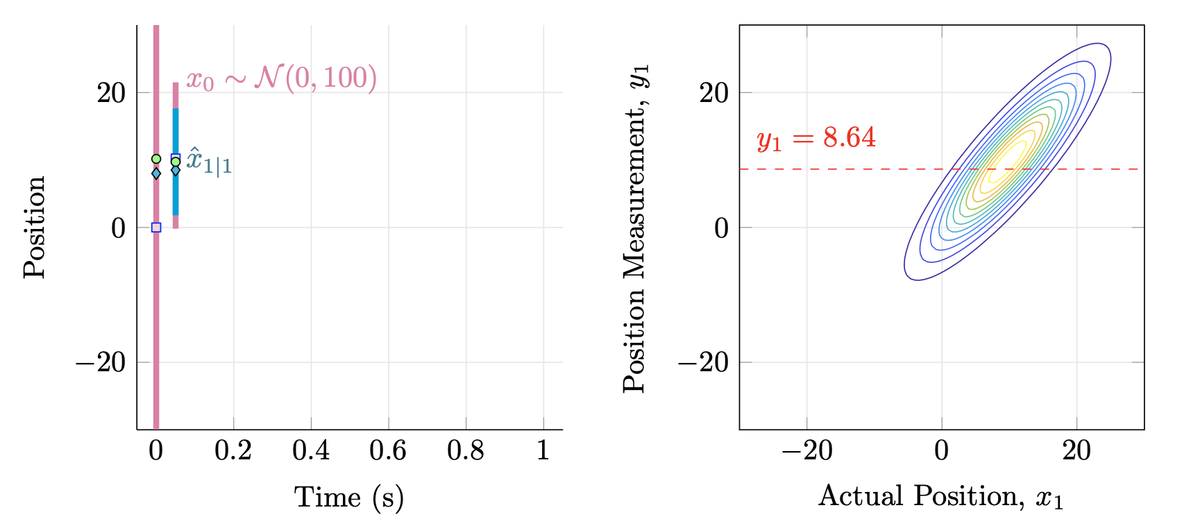
Figure IV.1. (Left) Estimated positions, $\hat{x}_{t\mid t-1}$ (pink square), $\hat{x}_{t\mid t}$ (blue rhombus) and the unknown true position (green circle). The vertical bars show the $\pm 3\sigma^2$-intervals around the estimated positions. (Right) Joint distribution of $(x_1, y_1)$ and a measurement $y_1=8.64$.
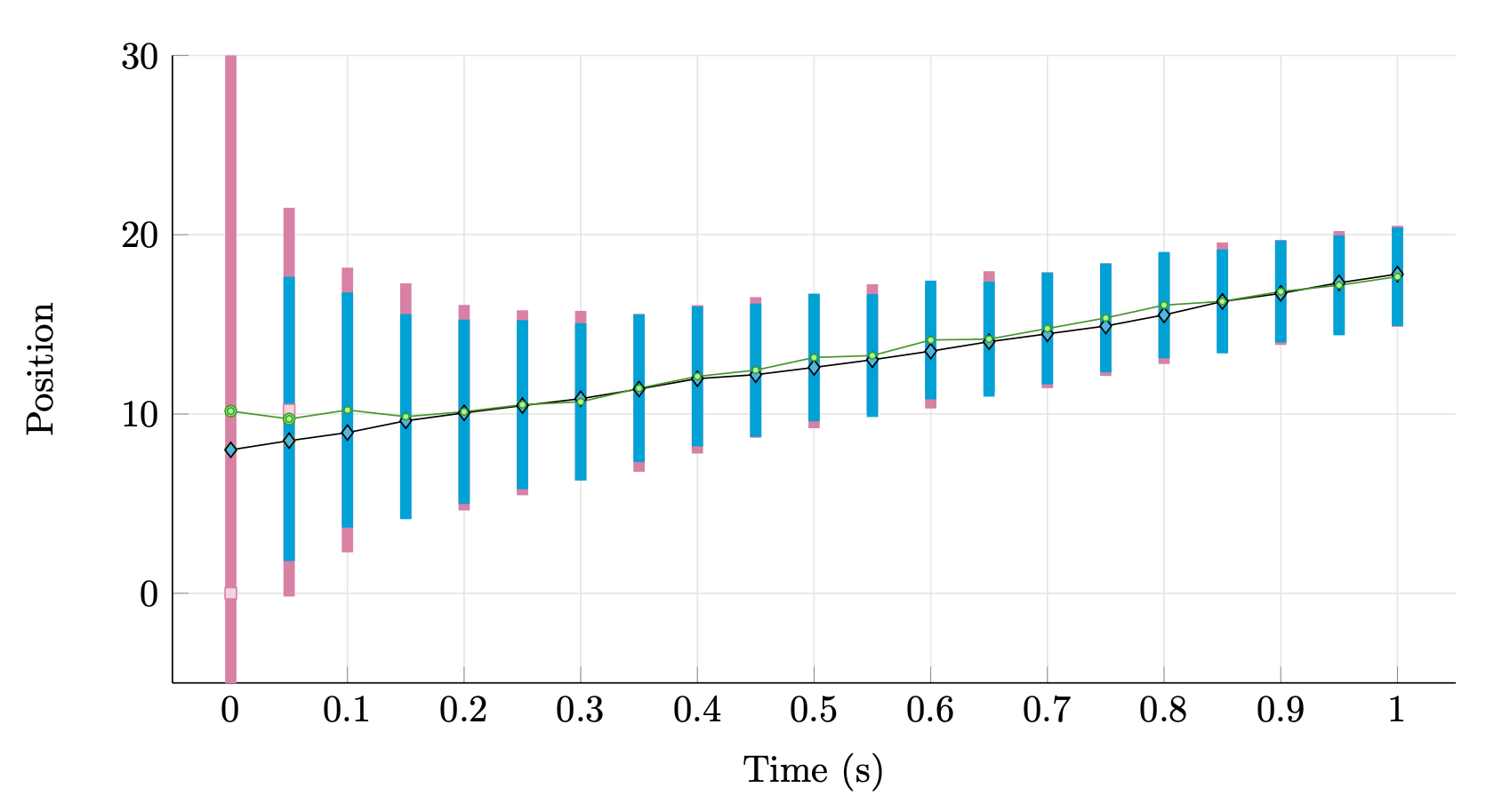
Figure IV.2. Estimated positions, $\hat{x}_{t\mid t-1}$ (pink square), $\hat{x}_{t\mid t}$ (blue rhombus) and the unknown true position (green circle). We observe that one new data becomes available, the variance of the estimated position decreases. We also see that $\Sigma_{t+1\mid t}$ converges to a finite variance and that in this example the estimation error is very small.
See also: Watch the following YouTube video
Intermittent measurements
Suppose we obtain measurements at $t=0,1,\ldots, t_1$, but then the connection to the GPS breaks so we have no measurements from $t_1+1$ to $t_2-1$. At time $t_2$ the connection is recovered. In that case, we can still apply the Kalman filter by applying only time update steps when we do not have measurements. This is illustrated in Figures IV.3 and IV.4.
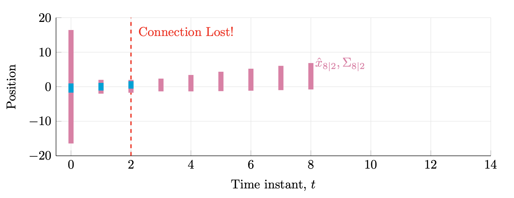
Figure IV.3. The connection is lost at $t_1=2$ and there are no measurements from time $3$ to time $7$; then, at $t_2=8$, the connection to the GPS is recovered (not shown here). Meanwhile, we compute the estimates $\hat{x}_{3{}\mid{}2},\ldots, \hat{x}_{8{}\mid{}2}$ and variances $\Sigma_{3{}\mid{}2},\ldots, \Sigma_{8{}\mid{}2}$.
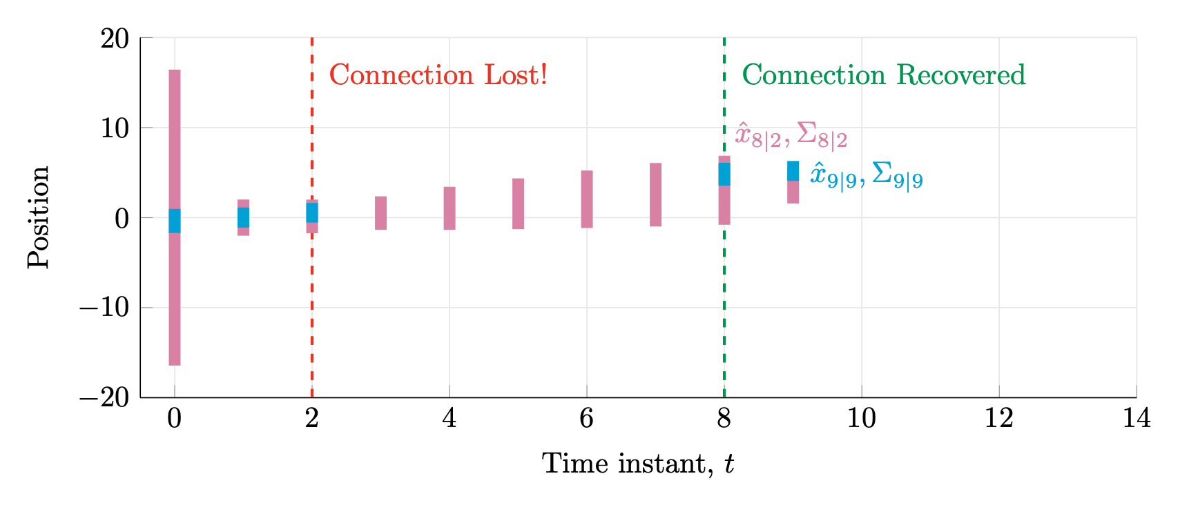
Figure IV.4. The connection is recovered at time $t_2=8$; subsequently, we can keep interleaving time and measurement update steps.
Read next: Kalman Filter V: It’s BLUE!