This is a draft of some lecture notes I prepared on principal component analysis. It is intended to be a gentle and smooth introduction to the topic. Some background in linear algebra is good to have, but we will take everything from the beginning.
1. The data matrix
1.1. Representation of the data
We have a matrix of data $X\in\R^{n\times p}$, i.e., we have $n$ measurements (experiments) with $p$ features.
For example, we have measured the age, $a$, weight, $b$, and height, $c$ of some people. We have $p=3$ features. We have the triples $(a_{(i)}, b_{(i)}, c_{(i)})$ for $i=1,2,\ldots, n$.
Notation: Hereafter, the subscript $(i)$, in parentheses, will refer to the $i$-th experiment (measurement). It is $i=1,\ldots, n$.
We denote each such triple by $x_{(i)} = (a_{(i)}, , b_{(i)}, c_{(i)})$ for $i=1,2,\ldots, n$. We now organise these data in a matrix as follows:
$$X = \begin{bmatrix} a_{(1)} & b_{(1)} & c_{(1)} \\ a_{(2)} & b_{(2)} & c_{(2)} \\ \vdots & \vdots & \vdots \\ a_{(n)} & b_{(n)} & c_{(n)} \end{bmatrix} {}={} \begin{bmatrix} x_{(1)}^\intercal \\ x_{(2)}^\intercal \\ \vdots \\ x_{(n)}^\intercal \end{bmatrix}.\tag{1}$$
This is the data matrix $X\in\R^{n\times p}$.
1.2. Expectation of the data
We have assumed that the expectation of all features is zero, therefore, with reference to our age-weight-height example above, we *assume* that we have
$$\underbrace{\tfrac{1}{n}\sum_{i=1}^{n}a_{(i)}}_{\text{sample mean of }a} = 0.\tag{2a}$$
Likewise,
$$\sum_{i=1}^{n}b_{(i)} = 0,\tag{2b}$$
and
$$\sum_{i=1}^{n}c_{(i)} = 0.\tag{2c}$$
1.3. Variance of the data
Given that the sample means of the data are zero, the sample variances are
$$s_{a}^2 = \tfrac{1}{n}\sum_{i=1}^{n}a_{(i)}^2,\tag{3a}$$
and, similarly,
$$\begin{aligned} s_{b}^2 {}={}& \frac{1}{n}\sum_{i=1}^{n}b_{(i)}^2, \\ s_{c}^2 {}={}& \frac{1}{n}\sum_{i=1}^{n}c_{(i)}^2. \end{aligned}\tag{3b,c}$$
Exercise: What are the sample covariances?
2. Linear Transformations
We want to transform that data, $x_{(i)}$, to some *new* data by defining *new* features. We will choose the new features to be a *linear combination* of the features we have.
Let us revisit the example with age-weight-height data and see how such a transformation may look like.
2.1. Example 1: change of units
Imagine that we measure $a$ in years, $b$ in kilograms, and $c$ in meters. Instead, we decide to measure $a$ in months. We define the new variable
$$\tilde{a} = 12a.\tag{4a}$$
We decide to measure $b$ in pounds, so we define
$$\tilde{b} = 2.20462b.\tag{4b}$$
Lastly, we decide to measure the height in yards, so we define
$$\tilde{c} = 1.09361c.\tag{4c}$$
Given a triple $x_{(i)} = (a_{(i)}, b_{(i)}, c_{(i)})$ we can easily determine the *new* features $\tilde{x}_{(i)}$. It is
$$\tilde{x}_{(i)} = (\tilde{a}_{(i)}, \tilde{b}_{(i)}, \tilde{c}_{(i)}) = (12a_{(i)}, 2.20462b_{(i)}, 1.09361c_{(i)}).\tag{5}$$
Let's see how the data looks like. The new data are shown in Figure 1 below.
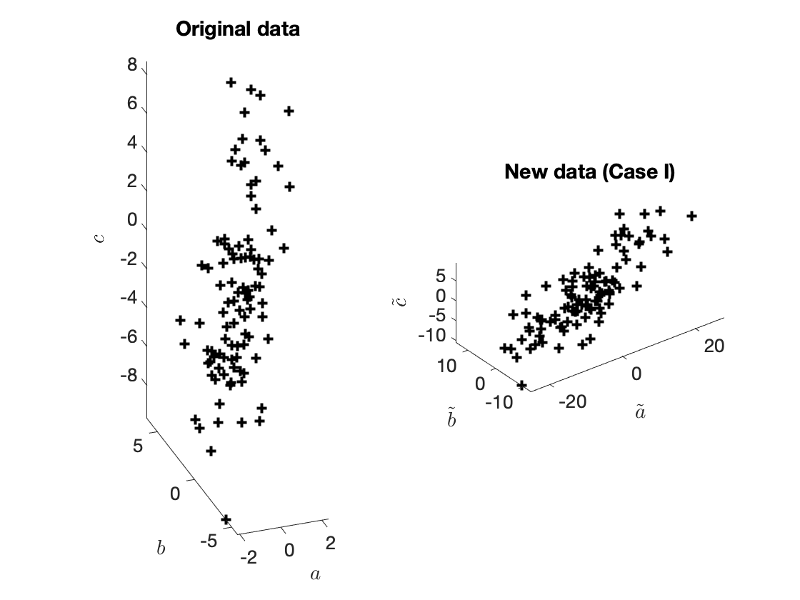
Figure 1. Original and new data.
2.2. Example 2: Apples + Oranges? Sure!
Let us now introduce the following new features. We define $$\tilde{a}_{(i)} = 0.2a_{(i)} + 0.2b_{(i)} + c_{(i)}.\tag{6a}$$ This new feature, is a linear combination of all three original features.
Likewise, we can define (utterly arbitrarily)
$$\tilde{b}_{(i)} = b_{(i)} - 0.2c_{(i)},\tag{6b}$$
and — why not
$$\tilde{c}_{(i)} = a_{(i)} - 0.2c_{(i)}.\tag{6c}$$
The new (transformed) data, $\tilde{x}_{(i)} = (\tilde{a}_{(i)}, \tilde{b}_{(i)}, \tilde{c}_{(i)})$ are shown below in Figure 2.
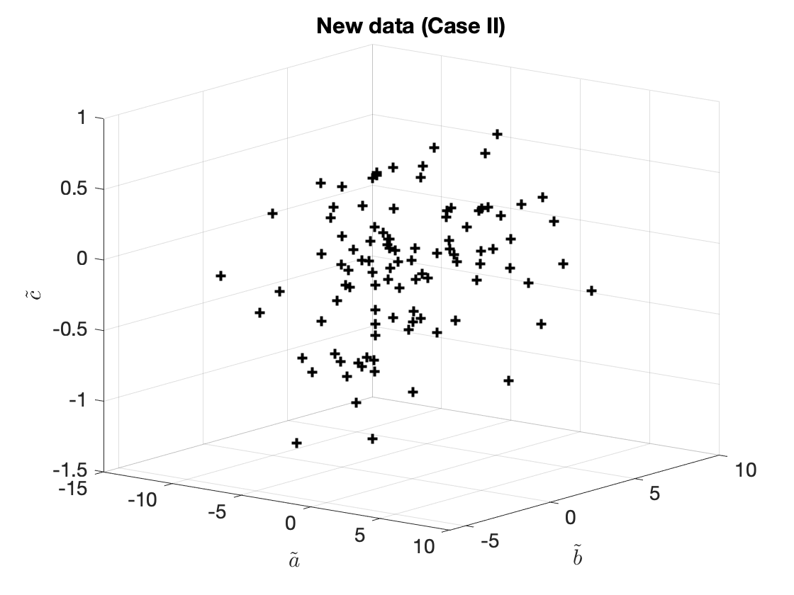
Figure 2. A different transformation.
2.3. Example 3: fewer features? why not!
The number of new features does not have to be the same as the number of original features. We can have fewer transformed features (even just one). For example, we can just define
$$\begin{aligned} \tilde{a}_{(i)} {}={}& 0.2a_{(i)} + 0.2b_{(i)} + c_{(i)}, \\ \tilde{b}_{(i)} {}={}&b_{(i)} - 0.2c_{(i)}, \end{aligned}\tag{7a,b}$$
and
$$\tilde{x}_{(i)} = (\tilde{a}_{(i)}, \tilde{b}_{(i)}).\tag{7c}$$
The (two-dimensional) transformed data are now shown in Figure 3.
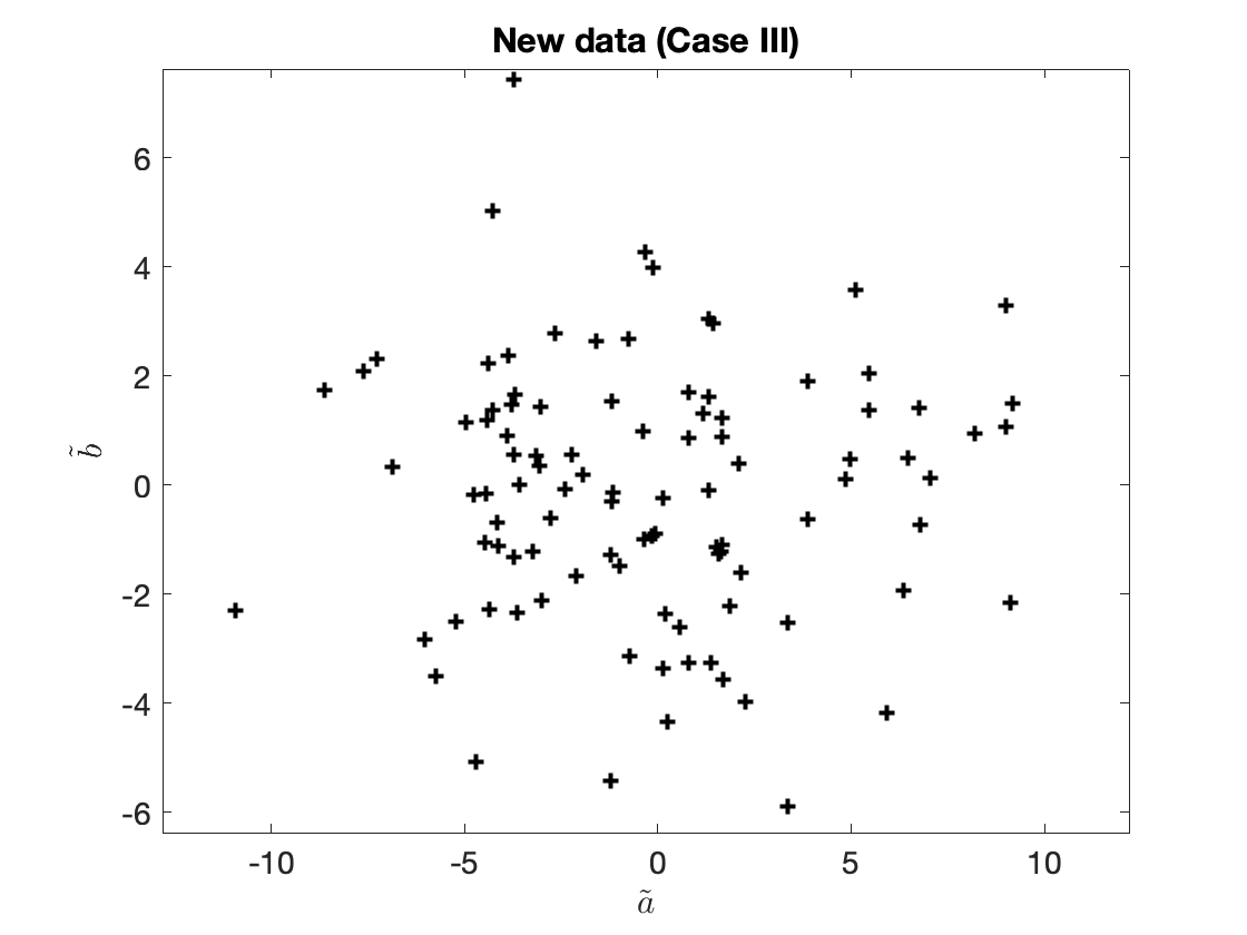
Figure 2. Transformed data (only two new features).
2.4. Example 4: more features? Sure!
We can also produce more features that the original ones. Back to our original example, we have the features $a_{(i)}, b_{(i)}, c_{(i)}$. We can define
$$\begin{aligned} \tilde{x}_{(i),1} {}={}& 3a_{(i)} + 2b_{(i)}, \\ \tilde{x}_{(i),2} {}={}& -10a_{(i)} - 8b_{(i)} - 11c_{(i)}, \\ \tilde{x}_{(i),3} {}={}& 6a_{(i)} + c_{(i)}, \\ \tilde{x}_{(i),4} {}={}& c_{(i)}, \\ \tilde{x}_{(i),5} {}={}& -b_{(i)}. \end{aligned}\tag{8a-e}$$
2.5. A general linear transformation
More generally, we have a linear transformation
$$x_{(i)} \mapsto \tilde{x}_{(i)},\tag{9}$$
with $x_{(i)} \in \R^p$ and $\tilde{x}_{(i)} \in \R^l$. It is a linear transformation $\R^p \to \R^l$.
Suppose that $x_{(i)}=(x_{(i),1}, x_{(i),2}, \ldots, x_{(i),p})$. Then,
$$\begin{aligned} \tilde{x}_{(i)1} {}={}& w_{1,1} x_{(i),1} + w_{1,2} x_{(i),2} + \ldots + w_{1,p} x_{(i),p}, \\ \tilde{x}_{(i)2} {}={}& w_{2,1} x_{(i),1} + w_{2,2} x_{(i),2} + \ldots + w_{2,p} x_{(i),p}, \\ \vdots\ \;{}& \\ \tilde{x}_{(i)l} {}={}& w_{l,1} x_{(i),1} + w_{l,2} x_{(i),2} + \ldots + w_{l,p} x_{(i),p}. \end{aligned}\tag{10}$$
Let us define
$$w_{j} = (w_{j, 1}, w_{j, 2}, \ldots, w_{j, p}),\tag{11}$$
for $j=1,\ldots, l$.
Then,
$$\begin{aligned} \tilde{x}_{(i)1} {}={}& \langle w_{1}, x_{(i)}\rangle , \\ \tilde{x}_{(i)2} {}={}& \langle w_{2}, x_{(i)}\rangle , \\ \vdots\ \;{}& \\ \tilde{x}_{(i)l} {}={}& \langle w_{l}, x_{(i)}\rangle . \end{aligned}$$
In other words, any linear transformation $\R^p \to \R^l$ can be described by $l$-many vectors $w_1,\ldots, w_l$ (where $w_j\in\R^p$).
Exercise: Go through Examples 1, 2, 3, and 4, and determine the vectors $w_j$ that describe the linear transformations.
What is this? We have the matrix $X\in\R^{n\times p}$ of original data. Take the vector $w_{1}\in\R^p$ we defined in Equations (11) and (12a). What is $$Xw_{1} = ?\tag{13}$$
3. Principle component analysis
3.1. The first component
Suppose we have applied a certain transformation to our original data and we have produced some new features. Suppose that the *first new feature* is $\tilde{x}_{(i), 1}$ and it is given by
$$\tilde{x}_{(i), 1} = \langle w_{1}, x_{(i)}\rangle .\tag{14}$$
Exercise: Show that the sample mean of the new feature is zero.
The first transformed variable, $\tilde{x}_{(i), 1}$, is identified by $w_1$. When choosing $w$ we have the following two objectives
- The norm of $w_1$ must be equal to $1$
- and $w_1$ should maximise its sample variance (as we say, $w_1$ is a maximiser of the variance of $\tilde{x}_{(i), 1}$).
We define $w_1$ to be
$$\begin{aligned} w_1^\star {}={}& \argmax\limits_{\|w_1\|=1}\;\text{ Sample variance of }\tilde{x}_{(i), 1} \\ {}={}& \argmax\limits_{\|w_1\|=1}\;\sum_{i=1}^{n}\tilde{x}_{(i), 1}^2 \\ {}={}& \argmax\limits_{\|w_1\|=1}\;\sum_{i=1}^{n} \langle w_1, x_{(i)}\rangle ^2 \\ {}={}& \argmax\limits_{\|w_1\|=1}\;\|Xw_1\|^2 \\ {}={}& \argmax\limits_{\|w_1\|=1}\;w_1^\intercal X^\intercal X w_1.\tag{15} \end{aligned}$$
Good news: we can solve this problem to determine $w^\star$: the matrix $X^\intercal X$ is symmetric, therefore, it has real eigenvalues, $\lambda_1 \leq \lambda_2 \leq \ldots \leq \lambda_{p}=\lambda_{\max}$, where $\lambda_{\max}$ is the maximum eigenvalue of $X^\intercal X$. Then, $w_1^\star$ is the corresponding eigenvector.
The vector $w_1^\star$ is shown in Figure 4.
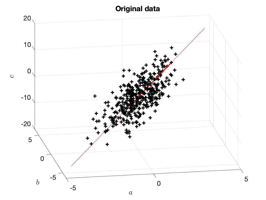
Figure 4. Original data and the vector $w_1^\star$. The thin red line shows the span of $w_1^\star$. The thicker red line shows $10\cdot w_1^\star$ (we have multiplied it by $10$ for it to be clearly visible).
If we chose any other vector $w_1'$ with $\|w_1'\|=1$, then the variance of $\tilde{x}_{(i), 1}$ would be lower. This is demonstrated in Figure 5.
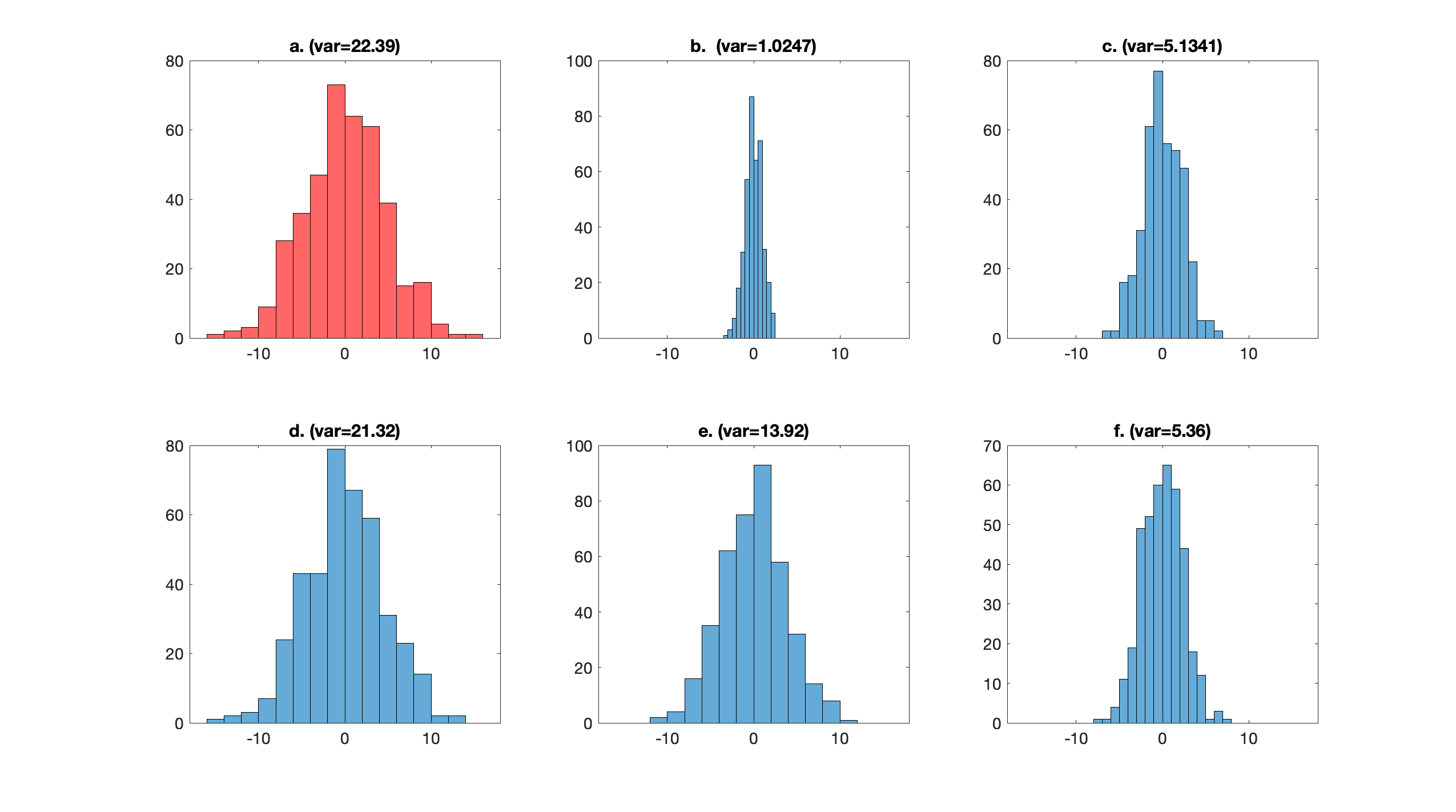
Figure 5. (a) Distribution of $\tilde{x}_{(i), 1} = \langle w_1^\star, x_{(i)}\rangle $, where $w_1^\star$ has been chose to be the eigenvector corresponding to the highest eigenvalue of $X^\intercal X$. The sample variance of $\tilde{x}_{(i), 1}$ is $22.39$. (b) Using $w_1 = (1, 0, 0)$, the variance is $1.0247$. (c) Using $w_1 = (0, 1, 0)$, the variance is $5.1341$. (d) Using $w_1 = (0, 0, 1)$, the variance is $21.32$. (e) Using $w_1 = \tfrac{\sqrt{3}}{3}(1, 1, 1)$, the variance is $13.92$. (f) Using $w_1 = \tfrac{\sqrt{3}}{3}(1, 1, -1)$, the variance is $5.36$. Having determined $w_1^\star$, we will now determine the second vector, $w_2^\star$.
3.2. The second component
Let $E_1$ be the set of vectors that are orthogonal to $w_1^\star$ as show in Figure 6.
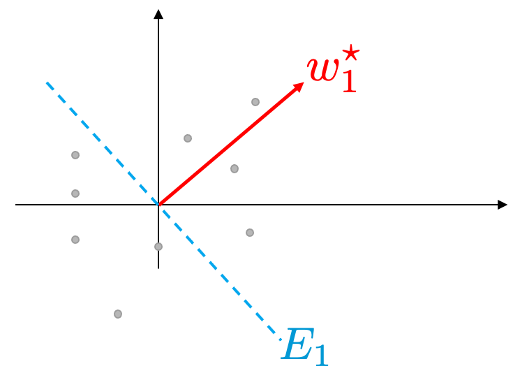
Figure 6. Our data (grey dots), the vector $w_1^\star$ which is determined as we discussed in the previous section, and the set $E_1$ of the vectors that are orthogonal to $w_1^\star$.
Next, we project all data points onto $E_1$ as shown in Figure 6.
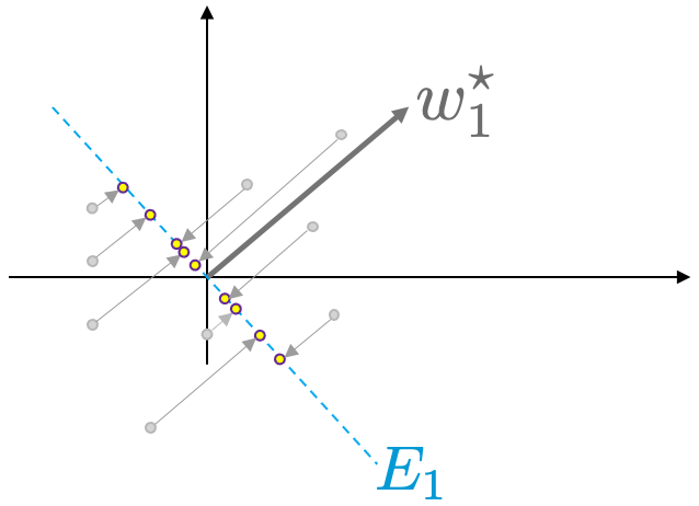
Figure 7. All data points, $x_{(i)}$ are projected on the space $E_1$.
There is a convenient formula that allows us to project all data points onto $E_1$. It is:
$$X_{E_1} = X - Xw_1^\star w_1^{\star\intercal}.\tag{16}$$
This returns a matrix $X_{E_1}\in\R^{n\times p}$ where all data points live in $E_1$; as such, they are orthogonal to $w_1^\star$.
In Figure 4 we saw how $w_1^\star$ looks like. In Figure 8 below we see the plane $E_1$.
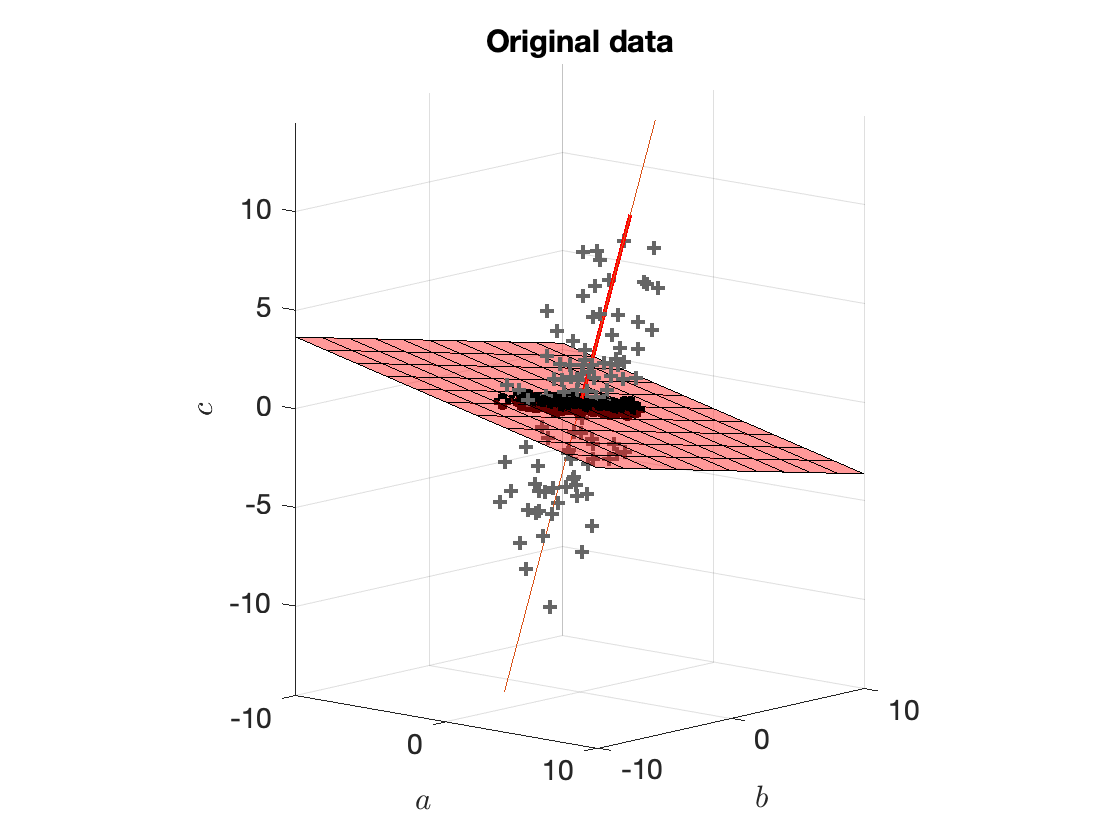
Figure 8. Original data points (grey crosses), vector $w_1^\star$ (red vector), plane $E_1$ (red surface), data projected onto $E_1$ (black circles). The vector $w_1^\star$ is orthogonal to $E_1$.
The vector $w_2^\star$ is chosen so as to satisfy the following conditions:
- $|w_2^\star| = 1$
- $w_2^\star\in E_1$, i.e., $w_2^\star$ is orthogonal to $w_1^\star$
- Focusing on the projected data on $E_1$, we want to maximise the variance of $X_{E_1}$ along the direction of $w_2^\star$. We choose $w_2^\star$ exactly as we chose $w_1^\star$: we take $w_2^\star$ to be the eigenvector that corresponds to the largest eigenvalue of $X_{E_1}X_{E_1}^\intercal$.
Figure 9 shows the second vector, $w_2^\star$.
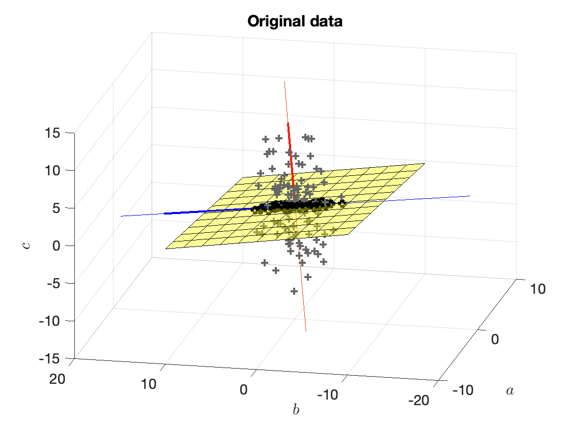
Figure 9. (Grey crosses) original points, (Red line) vector $w_1^\star$, (Blue line) vector $w_2^\star$, (Yellow surface) set $E_1$ of vectors that are orthogonal to $w_1^\star$.
Fact: The largest eigenvalue of $X_{E_1}X_{E_1}^\intercal$ (and the corresponding eigenvector) is the second-largest eigenvalue of $XX^\intercal$ (and the corresponding eigenvector).
3.3. The third component
The third vector, $w_3^\star$ is taken to be such that
- It has norm $1$
- It is orthogonal to both $w_1^\star$ and $w_2^\star$
- It maximises the variance of $X$ along the direction $w_3^\star$
4. Complete example
4.1. The data
We have the following synthetic (made up) data (original dataset $X$):
| Sepal Length ($x_1$) | Sepal Width ($x_2$) | Petal Length ($x_3$) | Petal Width ($x_{4}$) |
|---|---|---|---|
| -0.8977 | 1.0156 | -1.3358 | -1.3111 |
| -1.1392 | -0.1315 | -1.3358 | -1.3111 |
| -1.3807 | 0.3273 | -1.3924 | -1.3111 |
| -1.5015 | 0.0979 | -1.2791 | -1.3111 |
| -1.0184 | 1.2450 | -1.3358 | -1.3111 |
| -0.5354 | 1.9333 | -1.1658 | -1.0487 |
| -1.5015 | 0.7862 | -1.3358 | -1.1799 |
| -1.0184 | 0.7862 | -1.2791 | -1.3111 |
| -1.7430 | -0.3610 | -1.3358 | -1.3111 |
| … | … | … | … |
We have $n=150$ datapoints and $p=4$ features.
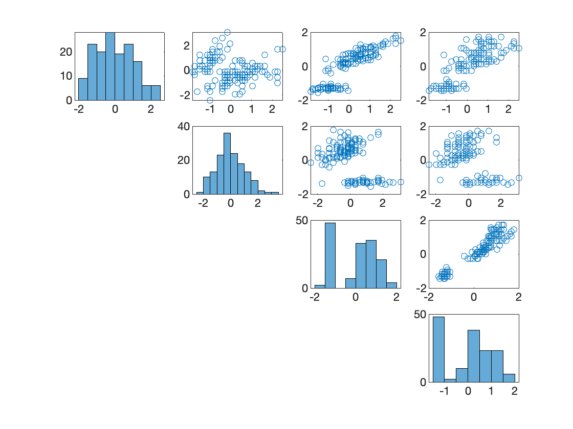
Figure 10. Correlations of the four variables in the original dataset. (Graphs on diagonal) histograms of $x_1$, $x_2$, $x_3$, and $x_4$. (Off-diagonal) The diagram in row $i$, column $j$, is a plot of $x_j$ (y-axis) vs $x_i$ (x-axis).
4.2. The principal components
The vectors $w_j^\star$, $j=1,\ldots, 4$, are given by
$$\begin{aligned} w_1^\star {}={}& (0.5211, -0.2693, 0.5804, 0.5649), \\ w_2^\star {}={}& (0.3774, 0.9233, 0.0245, 0.0669 ), \\ w_3^\star {}={}& (0.7196, -0.2444, -0.1421, -0.6343), \\ w_4^\star {}={}& (-0.2613, 0.1235, 0.8014, -0.5236). \end{aligned}$$
All these vectors have norm equal to 1 ($\|w_1^\star\|=\|w_2^\star\|=\|w_3^\star\|=\|w_4^\star\|=1$).
The four principal components (PCs) are
| PC | SepLength ($x_1$) | SepWidth ($x_2$) | PetLength ($x_3$) | PetWidth ($x_{4}$) | Eig/val |
|---|---|---|---|---|---|
| PC1 | 0.5211 | -0.2693 | 0.5804 | 0.5649 | 2.9185 |
| PC2 | 0.3774 | 0.9233 | 0.0245 | 0.0669 | 0.9140 |
| PC3 | 0.7196 | -0.2444 | -0.1421 | -0.6343 | 0.1468 |
| PC4 | -0.2613 | 0.1235 | 0.8014 | -0.5236 | 0.0207 |
This means that the principal components (new variables) are (fill in the missing values as an exercise)
$$\begin{aligned} \tilde{x}_1{}={}& 0.5211x_1 -0.2693x_2 + ?x_3 + ?x_4, \\ \tilde{x}_2 {}={}& ?x_1 + ?x_2 + ?x_3 + ?x_4, \\ \tilde{x}_3 {}={}& ?x_1 + ?x_2 + ?x_3 + ?x_4, \\ \tilde{x}_4 {}={}& ?x_1 + ?x_2 + ?x_3 + ?x_4. \end{aligned}$$
The eigenvalue that corresponds to PC1 ($\tilde{x}_1$) is approximately 2.9; it is noticeably larger than all other eigenvalues. Also the eigenvalues of PC3 and PC4 can be considered negligible (designer's choice; it's up to you. I'm not sure whether there are widely adopted standards). The eigenvalues are shown also in Figure 11.
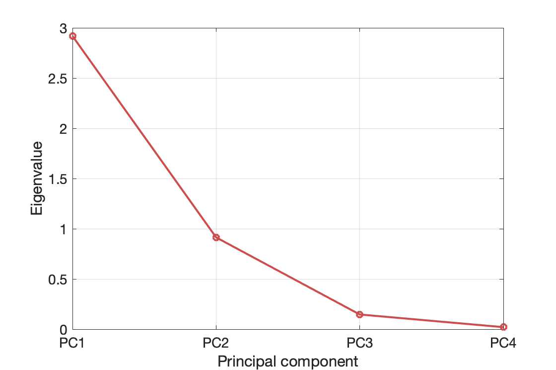
Figure 11. Principal components and their eigenvalues.
4.4. What do the eigenvalues really mean?
The eigenvalues that correspond to the PCs are a measure of the significance of the PCs. Let's be more specific...
What do the eigenvalues mean? The sample variance of $\tilde{x}_i$ (the $i$-th principal component) is equal to the eigenvalue that corresponds to that PC.
4.5. Le biplot
We’ve seen that the first two PCs are quite dominant. We will treat the other two PCs as insignificant and we’ll ignore them.
We want to understand how the two most dominant PCs depend on the original features.
Let us have another look at the coefficients…
| PC | SepLength ($x_1$) | SepWidth ($x_2$) | PetLength ($x_3$) | PetWidth ($x_{4}$) |
|---|---|---|---|---|
| PC1 | 0.5211 | -0.2693 | 0.5804 | 0.5649 |
| PC2 | 0.3774 | 0.9233 | 0.0245 | 0.0669 |
Enter Biplot… A biplot is a plot showing (i) two of the principal components (typically PC1 and PC2), (ii) the contributions of the original variables to the PCs.
Let us have a look at the biplot of Figure 12.
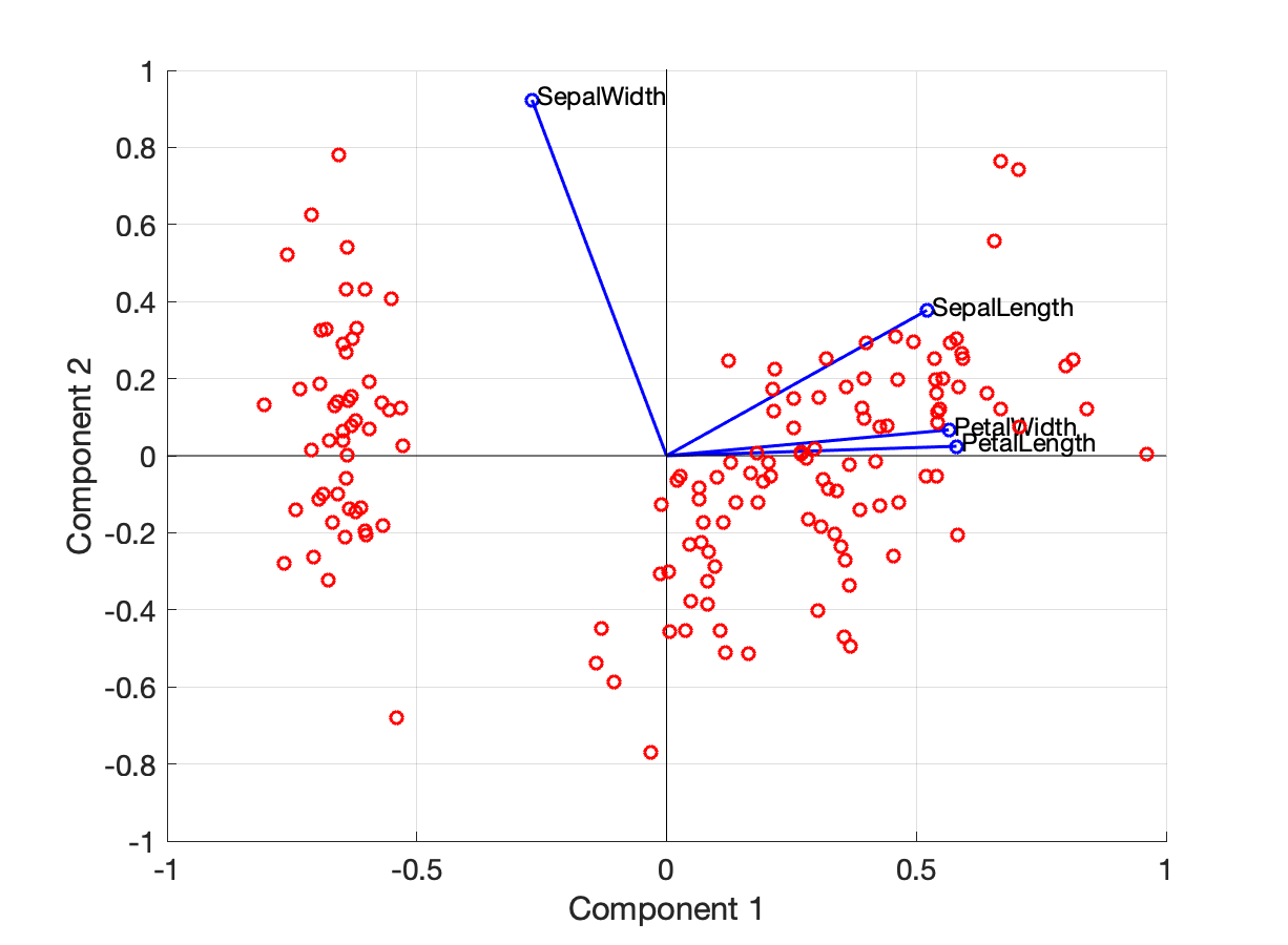
Figure 12. Biplot with PC1 and PC2. (Red dots) PC1 and PC2 of the data ($\tilde{x}_1$ and $\tilde{x}_2$). The blue vectors show how much each of the original variables contributes to the PCs. For example the (blue) vector that correspond to `SepalWidth` is $(-0.2693, 0.9233)$.
In Figure 12 we see that:
- The blue arrows are not too small (all of them have a length between 0.5 and 1). $\implies$ All original variables have a non-negligible contribution to the PCs
- SepalWidth affects PC1 with a negative coefficient (-0.2693) and PC2 with a positive coefficient (0.9233)
- SepalLength affects both PC1 and PC2 with a positive coefficient
- PetalLength and PetalWidth do not affect PC2 too significantly
For completeness, here is the biplot with PC3 and PC4:
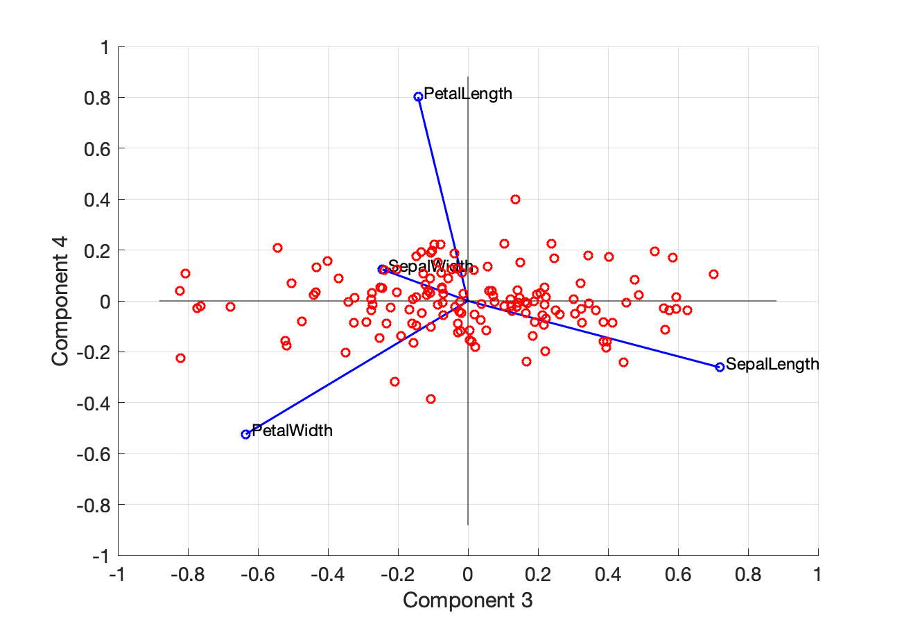
Figure 13. Biplot with PC3 and PC4.
Note: An important note is that the covariance between two PCs is zero.
4.6. MATLAB code
First, we load the data
set(0, 'DefaultTextFontSize',12)
set(0, 'DefaultAxesFontSize', 14)

load fisheriris
Z = zscore(meas);
Then, compute the PCA
[coefs,scores, lat] = pca(Z);
Correlogram:
for i=1:4
    idx = 5*i-4;
    subplot(4, 4, idx);
    histogram(Z(:, i));
    for j=1:4-i
        subplot(4, 4, idx+j);
        plot(Z(:, i), Z(:, i+j), 'o')
    end
end
Plot the eigenvalues of the PCs
plot([1, 2, 3, 4],lat, '-o', 'linewidth', 2, 'Color', [0.8, 0.3, 0.3])
xticks([1, 2, 3, 4])
xticklabels({'PC1','PC2','PC3','PC4'})
ylabel('Eigenvalue')
xlabel('Principal component')
Biplot:
figure('Units','normalized','Position',[0.3 0.3 0.3 0.5])
variables = {'SepalLength','SepalWidth','PetalLength','PetalWidth'};
biplot(coefs(:,1:2),'Scores',scores(:,1:2),...
    'VarLabels',variables,...
    'Marker','o', 'linewidth', 1.5);
xlim([-1 1]); ylim([-1 1]);
5. Relationship to SVD
PCA is related to the singular value decomposition (SVD) of the data matrix $X$,
$$X = USV^\intercal.$$
We can see that
$$X^\intercal X = VS^\intercal U^\intercal U S V^\intercal = V(S^\intercal S) V^\intercal.$$
The matrix $S^\intercal S$ is square and diagonal and the columns of $V$ are the eigenvectors of $X^{\intercal} X$. This means that $V = W$ (the PCA transformation).
The PCs are given by
$$\widetilde{X} = XW = XV = US.$$
This is a form of polar decomposition of $X$.