In this introductory post we will present some fundamental results that will pave the way towards polynomial chaos expansions. This will be done in a series of blog posts.
0. Introduction
0.1. Preliminaries
Mercer's theorem is a fundamental theorem in reproducing kernel Hilbert space[ref]. Before we proceed we need to state a few definitions. Note certain authors use different notation and definitions. We start with the definition of a symmetric function.
Definition 1 (Symmetric). A function \(K:[a,b]\times[a,b] \to {\rm I\!R}\) symmetric if $K(x, y) = K(y, x)$ for all $x,y\in[a,b]$.
Next we give the definition of a positive definite function \(K:[a,b]\times[a,b] \to {\rm I\!R}\).
Definition 2 (Positive definite function). A function \(K:[a,b]\times[a,b] \to {\rm I\!R}\) is called nonnegative definite if \(\sum_{i,j=1}^{n} f(x_i) f(x_j) K(x_i,x_j) \geq 0\), for all \((x_i)_{i=1}^{n}\) in \([a,b]\), all \(n\in\N\) and all functions \(f:[a, b] \to {\rm I\!R}\).
We can now give the definition of a kernel.
Definition 3 (Kernel). A function \(K:[a,b]\times[a,b] \to {\rm I\!R}\) is called a kernel if it is (i) continuous, (ii) symmetric, and (iii) nonnegative definite.
Some examples of kernels are (for $x,y\in [a, b]$)
- Linear, $K(x, y) = x y$
- Polynomial, $K(x, y) = (x y + c)^d$, with $c\geq 0$
- Radial basis function, $K(x, y) = \exp(-\gamma (x-y)^2)$
- Hyperbolic tangent, $K(x, y) = \tanh(xy + c)$
0.2. Hilbert-Schmidt integral operators
We give the definition of the Hilbert-Schmidt integral operator of a kernel.
Definition 4 (HS integral operator). Let \(K\) be a kernel. The Hilbert-Schmidt integral operator is defined as a $T_K : \mathcal{L}^2([a,b]) \to \mathcal{L}^2([a,b])$ that maps a function $\phi \in \mathcal{L}^2([a,b])$ to the function
$$T_K \phi = \int_{a}^{b}K({}\cdot{}, s)\phi(s)\mathrm{d} s.$$
which is an $\mathcal{L}^2([a,b])$-function.
The Hilbert-Schmidt integral operator of a kernel is linear, bounded, and compact. Moreover, $T_K\phi$ is continuous for all $\phi\in\mathcal{L}^2([a,b])$. We also have that $T_K$ is self adjoint, that is, for all $g\in\mathcal{L}^2([a,b])$,
$$\langle T_K \phi, g\rangle = \langle \phi, T_K g\rangle.$$
Recall that given a linear map $A:U\to U$ on a real linear space $U$, an eigenvalue-eigenvector pair $(\lambda, \phi)$, with $\lambda\in\mathbb{C}$ and $\phi\in U$ is one that satisfies $A\phi = \lambda \phi$.For the Hilbert-Schmidt integral operator of a kernel
- There is at least one eigenvalue-eigenfunction pair
- The set of its eigenvalues is countable
- Its eigenvalues are (real and) nonnegative
- Its eigenfunctions are continuous
- Its eigenfunctions span $\mathcal{L}^2([a,b])$
From the spectral theorem for linear, compact, self-adjoint operators, there is an orthonormal basis of $\mathcal{L}^2([a,b])$ consisting of eigenvectors of $T_K$.
0.3. Mercer’s Theorem
We can now state Mercer's theorem.
Theorem 5 (Mercer's theorem). Let \(K\) be a kernel. Then, there is an orthonormal basis \((e_i)_{i}\) of $\mathcal{L}^2([a,b])$ of eigenfunctions of $T_K$, and corresponding (nonnegative) eigenvalues \((\lambda_i)_i\) so that
$$K(s,t) = \sum_{j=1}^{\infty} \lambda_j e_j(s)e_j(t),$$
where convergence is absolute and uniform in \([a,b]\times [a,b]\).
The fact that $(\lambda_i, e_i)$ is an eigenvalue-eigenfunction pair of $T_K$ means that $T_K e_i = \lambda_i e_i$, that is,
$$\int_a^b K(t, s)e_i(s)\mathrm{d}s = \lambda_i e_i(t).$$
This is a Fredholm integral equation of the second kind.
1. The Kosambi–Karhunen–Loève Theorem
We can now state the Kosambi–Karhunen–Loève (KKL) theorem[3]. The Kosambi–Karhunen–Loève Theorem is a special case of the class of polynomial chaos expansions we will discuss later. It is a consequence of Mercer's Theorem.
Theorem 6 (KKL Theorem).[3] Let \((X_t)_{t\in [a,b]}\) be a centred, continuous stochastic process on \((\Omega, \mathcal{F}, \mathrm{P})\) with a covariance function $R_X(s,t) = {\rm I\!E}[X_s X_t]$. Then, for $t\in[a, b]$
\[ X_t(\omega) = \sum_{i=1}^{\infty}Z_i(\omega) e_i(t),\tag{1} \]
with
\[ Z_i(\omega) = \int_{T}X_t(\omega)e_i(t) \mathrm{d}t, \tag{2} \]
where $e_i$ are eigenfunctions of the Hilbert-Schmidt integral operator of $R_X$ and form an orthonormal basis of $\mathcal{L}^2(\Omega, \mathcal{F}, \mathrm{P})$.
Since $(Z_i)_i$ is an orthonormal basis, \({\rm I\!E}[Z_i Z_j] = 0\) for \(i\neq j\). Moreover, \({\rm I\!E}[Z_i]=0\). The variance of $Z_i$ is ${\rm I\!E}[Z_i^2] = \lambda_i$ — the corresponding eigenvalue to $Z_i$.
In Equation (1), the series converges in the mean-square sense to $X_t$, uniformly in $t\in[a,b]$.
What is more, \((e_i)_i\) and \((\lambda_i)_i\) are eigenvectors and eigenvalues of the Hilbert-Schmidt integral operator \(T_{R_X}\) of the auto-correlation function \(R_X\) of the random process, that is, they satisfy the Fredholm integral equation of the second kind
\[ T_{R_X}e_i = \lambda_i e_i \]
or equivalently
\[ \int_{a}^{b} R_X(s,t) e_i(s) \mathrm{d} s = \lambda_i e_i(t), \]
for all $i\in\N$.
Let \((X_t)_{t\in T}\), \(T=[a,b]\), be a stochastic process which satisfies the requirements of the Kosambi-Karhunen-Loève theorem. Then, there exists a basis \((e_i)_i\) of \(\mathcal{L}^2(T)\) such that for all \(t\in T\)
\[ X_t(\omega) = \sum_{i=1}^{\infty} \sqrt{\lambda_i}\xi_i(\omega)e_i(t), \]
in \(\mathcal{L}^2(\Omega, \mathcal{F}, \mathrm{P})\), where \(\xi_i\) are centered, mutually uncorrelated random variables with unit variance and are given by
\[\xi_i(\omega) = \tfrac{1}{\sqrt{\lambda_i}}\int_{a}^{b} X_{\tau}(\omega) e_i(\tau) \mathrm{d} \tau.\]
2. Orthogonal polynomials
Let \(\mathsf{P}_N([a,b])\) denote the space of polynomials \(\psi:[a,b]\to{\rm I\!R}\) of degree no larger than \(N\in\N\).
Consider the space \(\mathcal{L}^2([a,b])\) and a positive continuous random variable with pdf $w$ (or, in general, a positive function $w:[a, b] \to [0, \infty)$). For two functions \(\psi_1,\psi_2: [a,b] \to {\rm I\!R}\), we define the scalar product
\[ \left\langle\psi_1, \psi_2\right\rangle_{w} = \int_{a}^{b} w(\tau) \psi_1(\tau) \psi_2(\tau) \mathrm{d} \tau. \]
and the corresponding norm \( \|f\|_w = \sqrt{\left\langle f,f\right\rangle_w}\). Define the space
\[ \mathcal{L}^2_w([a,b]) = \{f:[a,b]\to{\rm I\!R} {}:{} \|f\|_w < \infty\}. \]
For a random variable \(\Xi \in \mathcal{L}^2(\Omega, \mathcal{F}, \mathrm{P}; {\rm I\!R})\) with PDF \(p_\Xi>0\), we define
\[ \left\langle\psi_1, \psi_2\right\rangle_{\Xi} {}\coloneqq{} \left\langle\psi_1, \psi_2\right\rangle_{p_{\Xi}}. \]
If the random variable $\Xi$ is not continuous (so, it does not have a pdf), then given its distribution $F_{\Xi}(\xi) = \mathrm{P}[\Xi \leq \xi]$, we can define the inner product as
$$\langle \psi_1, \psi_2\rangle_{\Xi} {}={} \int_{a}^{b}\psi_1 \psi_2 \mathrm{d}F_{\Xi}.$$
Let $\Xi$ be a real-valued random variable with probability density function $p_\Xi$. Let \(\psi_1,\psi_2:\Omega\to{\rm I\!R}\) be two polynomials. We say that \(\psi_1,\psi_2\) are orthogonal with respect to (the pdf of) \(\Xi\) if \(\left\langle\psi_1, \psi_2\right\rangle_{\Xi} = 0\).
The random variable $\Xi$ the induces the above inner product and norm is often referred to as the germ.
Let \(\psi_0, \psi_2,\ldots\), with \(\psi_0=1\), be a sequence of orthogonal polynomials with respect to the above inner product. Then,
\[ 0 = \left\langle \psi_0, \psi_1 \right\rangle_\Xi = \int_{-\infty}^{\infty} \psi_{1}(s) p_{\Xi}(s) \mathrm{d} s = {\rm I\!E}[\psi_1(\Xi)], \]
by virtue of LotUS. Likewise, \({\rm I\!E}[\psi_i(\Xi)] = 0\) for all \(i\).
2.1. Popular polynomial bases
(Hermite polynomials). Let \(\Xi\) be distributed as \(\mathcal{N}(0,1)\). Then, its pdf is
$$p_{\Xi}(s) = \frac{1}{\sqrt{2\pi}}e^{-\frac{x^2}{2}}.$$
and the polynomials \(\psi_0,\psi_1,\ldots\) are the Hermite polynomials, the first few of which are \(H_0(x)=1\), \(H_1(x)=x\), \(H_2(x)=x^2-1\), \(H_3(x) = x^3 - 3x\). These are orthogonal with respect to \(\Xi\), that is
\[ \left\langle{}H_i, H_j\right\rangle_\Xi = \int_{-\infty}^{\infty}H_i(s) H_j(s) e^{-\frac{s^2}{2}}\mathrm{d} s = 0, \]
for \(i\neq j\).
(Legendre polynomials). If \(\Xi\sim U([-1,1])\), then \(\psi_0,\psi_1,\ldots\) are the Legendre polynomials. If, instead, \(\Xi\sim U([-1,1])\), the coefficients of the Legendre polynomials can be modified.
(Laguerre polynomials). If the germ is an exponential random variable on \([0,\infty)\), then \(\psi_0,\psi_1,\ldots\) are the Laguerre polynomials.
2.2. Projection and Best Approximation
On a normed space $X$, let us recall that the projection of a point $x \in X$ on a closed set $H\subseteq X$ is defined as
$$\Pi_H(x) = \argmin_{y\in H}\|y-x\|.$$
In other words,
$$\|\Pi_H(x) - x\| \leq \|y-x\|, \text{ for all } y\in H.$$
Proposition 7 (Projection on subspace). Let $X$ be an inner product space and $H \subseteq X$ is a linear subspace of $X$. Let $x\in X$. The following are equivalent
- $x^\star = \Pi_{H}(x)$
- $\|x^\star - x\| \leq \|y-x\|$, for all $y\in H$
- $x^\star - x$ is orthogonal to $y$ for all $y\in H$
Proof. (1 $\Leftrightarrow$ 2) is immediate from the definition of the projection.
(1 $\Leftrightarrow$ 3) The optimisation problem that defines the projection can be written equivalently as
$$\operatorname*{Minimise}_{y}\tfrac{1}{2}\|y-x\|^2 + \delta_H(y).$$
So the optimality conditions are $0 \in \partial(\tfrac{1}{2}\|x^{\star}-x\|^2 + \delta_H(x^{\star}))$. Equivalently
$$0 \in x^{\star}-x + N_H(x^{\star}) \Leftrightarrow x^{\star}-x \in H^{\perp},$$
and this completes the proof. $\Box$
Proposition 8 (Projection on subspace). Let $X$ be an inner product space and $H \subseteq X$ is a finite-dimensional linear subspace of $X$ with an orthogonal basis $\{e_1, \ldots, e_n\}$*. Then,
$$\Pi_H(x) = \sum_{i=1}^{n}c_i e_i,$$
where
$$c_i = \frac{\langle x, e_i \rangle}{\|e_i\|^2},$$
for all $i=1,\ldots, n$.
* If the basis is not orthogonal, we can produce an orthogonal basis using the Gram-Schmidt orthogonalisation procedure[ref]
Proof. It suffices to show that Condition 3 of Proposition 7 is satisfied. Equivalently, it suffices to show that
$$\left\langle \sum_{i=1}^{n} \frac{\langle x, e_i \rangle}{\|e_i\|^2}e_i - x, e_j\right\rangle=0,$$
for all $j=1,\ldots,n$. This is true because $\langle e_i, e_j\rangle = \delta_{ij}\|e_j\|^2$. $\Box$
Let $\{\psi_0, \ldots, \psi_N\}$ be an orthogonal basis of the set of polynomials on $[a, b]$ with degree up to $N$. This is denoted by $\mathsf{P}_N([a, b])$. Orthogonality is meant with respect to an inner product \(\left\langle{}\cdot{}, {}\cdot{}\right\rangle_w\). Suppose that the $\psi_i$ are unitary, i.e., $\|\psi_i\|_w = 1$.
Following Proposition 8, the projection operator onto \(\mathsf{P}_N([a, b])\) is
\[ \Pi_N:\mathcal{L}^2_w([a, b]) \ni f \mapsto \Pi_N f \coloneqq \sum_{j=0}^{N}\hat{f}_j \psi_j \in \mathsf{P}_N, \]
where $\hat{f}_j = \left\langle{}f, \psi_j\right\rangle_w.$
For \(f\in\mathcal{L}^2_w([a, b])\), define \(f_N = \Pi_N f\). Then,
\[ \lim_{N\to\infty}\|f - f_N\|_{w} = 0. \]
2.3. Example
Here we will approximate the function
$$f(x) = \sin(5x) \exp(-2x^2),$$
over $[-1, 1]$ using Legendre polynomials[ref]. The Legendre polynomials, $L_0, L_1, \ldots$ are orthogonal with respect to the standard inner product of $\mathcal{L}^2([-1, 1])$. The first four Legendre polynomials are
$$\begin{aligned} L_0(x) {}={}& 1, \\ L_1(x) {}={}& x, \\ L_2(x) {}={}& \tfrac{1}{2}(3x^2 - 1), \\ L_3(x) {}={}& \tfrac{1}{2}(5x^3 - 1). \end{aligned}$$
Using Proposition 8, we can compute the coefficients of the approximation $f \approx \Pi_N f$. In Figure 1 we see a comparison of $f_5$, $f_7$ and $f_9$ with $f$. We see that as $N$ increases, the approximation comes closed to $f$.
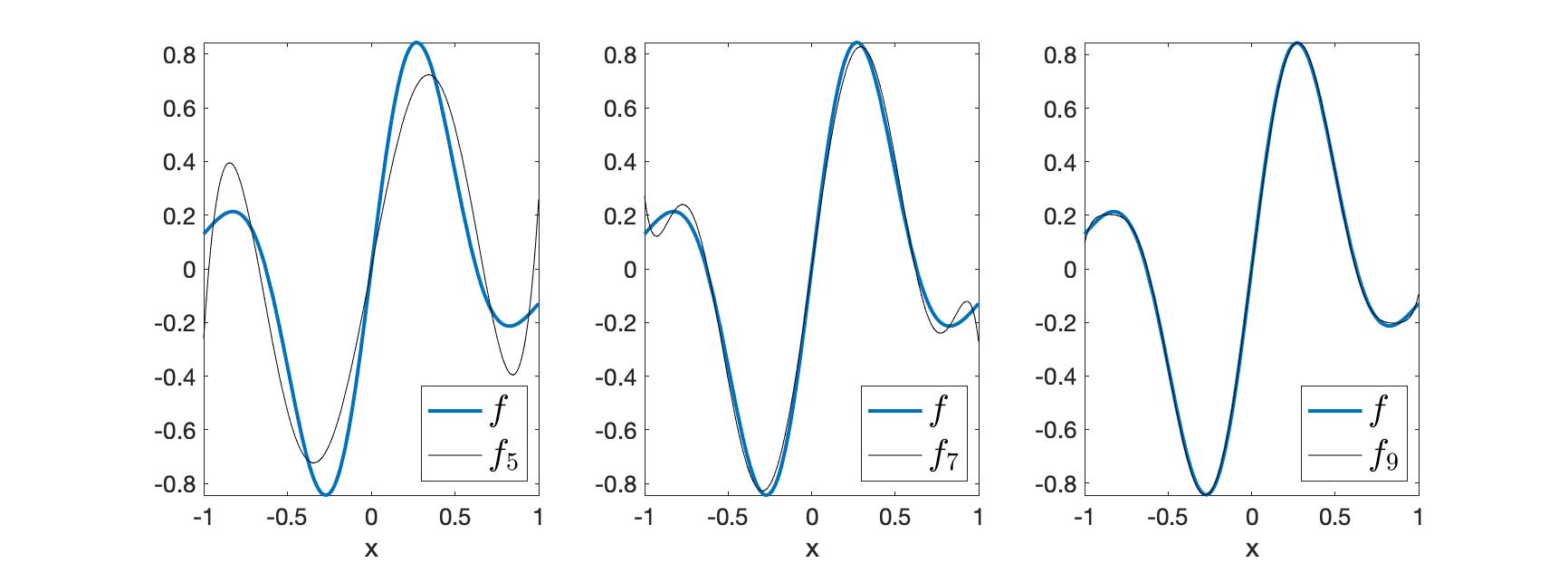
Figure 1. Approximation of $f(x) = \sin(5x) \exp(-2x^2)$ using Legendre polynomials.
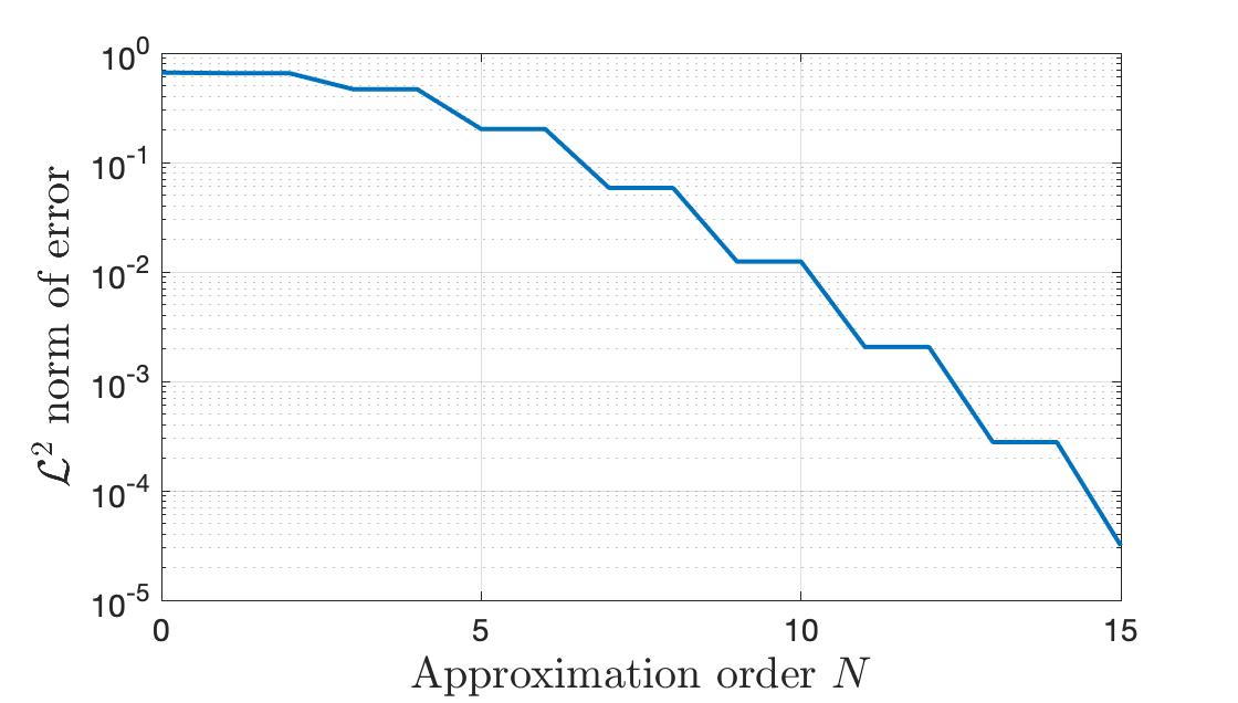
Figure 2. Plot of $\|f-f_N\|_{\mathcal{L}^2([-1, 1])}$ against $N$. As $N\to\infty$, the approximation error goes to zero.
Is this better compared to the Taylor expansion? TL;DR: Yes! Big time! Taylor's approximation is a local approximation.
2.4. Focused approximation
Let's take the same function as in the example of Section 2.3, but now suppose we want to focus more close to $-1$ and less so close to $1$. We want to treat errors close to $-1$ as more important and errors closer to $1$ as less important. To that end, we use the weight function
$$w(x) = (1-x)^a(1+x)^b,$$
with $a=2$ and $b=0.1$.
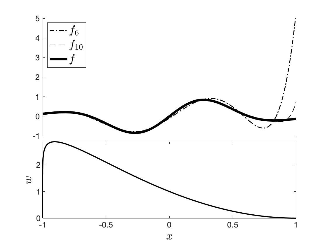
Figure 3. Approximation of $f(x) = \sin(5x) \exp(-2x^2),$ with polynomials which are orthogonal with respect to $w$.
The Jacobi polynomials[ref] are orthogonal with respect to $w$.
In Figure 3 we see that the approximation using an expansion with Jacobi polynomials is better close to $-1$ and less so as we move to $1$.
Read next
References
- G.E. Fasshauer, Positive Definite Kernels: Past, Present and Future, 2011
- Marco Cuturi, Positive Definite Kernels in Machine Learning, 2009
- R.B. Ash, Information Theory, Dover Books on Mathematics, 2012
- D. Xiu, Numerical methods for stochastic computations: a spectral method approach, Princeton University Press, 2010